MCMCtree

Overview

The program MCMCtree may be the first Bayesian phylogenetic program (Yang and Rannala 1997; Rannala and Yang 1996), but was very slow and decommissioned since the release of MrBayes (Huelsenbeck and Ronquist 2001). Since PAML version 3.15 (Yang 2000), MCMCtree implements the MCMC algorithms of Yang and Rannala (2006) and then of Rannala and Yang (2007) for estimating species divergence times on a given rooted tree using multiple fossil calibrations. These features are similar to the multidivtime program of Jeff Thorne and Hiro Kishino (see Thorne and Kishino 2002). The differences between the two programs are discussed by Yang and Rannala (2006) and Yang (2006, Section 7.4); see also below.

Please refer to any book on Bayesian computation for the basics of MCMC algorithm (e.g., chapters 6 and 7 in Yang 2014). Below, you may find some notes about MCMCtree:

Before starting the program on your PC, you may want to resize the window to have 100 columns instead of 80 (e.g., you can increase/decrease the size of your terminal accordingly so that some parts of the output file read better). If you are running MCMCtree on a High-Performance Computing (HPC) cluster or you do not intend to visually keep track of the screen output on a terminal, you do not need to worry about this.
The tree in Newick format that you should include in your input tree file must be a rooted binary tree: every internal node should have exactly two daughter nodes. You should not use a consensus tree with polytomies for divergence time estimation using MCMCtree. Instead, you should use a bifurcating ML tree or NJ tree or traditional morphology tree.
The tree in Newick format must not have branch lengths. For example, ((a:0.1, b:0.2):0.12, c:0.3) '>0.8<1.0'; does not work, while ((a, b), c) '>0.8<1.0'; (equivalent to ((a, b), c) 'B(0.8,1.0)'; or ((a, b), c) 'B(0.8,1.0,0.025,0.025)';) is fine. Below, you will learn more about the MCMCtree notation you need to follow when specifying node age constraints in your input tree file.
Under relaxed-clock models (i.e., setting clock = 2 or clock = 3 in the control file, more details later under the "Control file" section), the root age must always be constrained. In versions older than v4.10.7, you may have been specifying the root age constraint by using variable RootAge in the control file. Now, the root age constraint should be specified in the Newick tree file alongside the rest of node age constraints, which should reduce issues with the tree file format. When you use clock = 1 (i.e., the strict clock model is enabled), there should be no need to include a node age constraint for the root, but the program insists that you have it. In other words, regardless of the clock model you want to specify with variable clock, please constrain the root age of the tree topology you have included in your input tree file.

Warning

The suggestions above only apply to nucleotide, codon, and protein data. If you are using morphological quantitative data and enabling variable TipDate (i.e., you have included fossil taxa in your morphological alignment, which will be linked to an estimated age), please note that variable RootAge must be specified in the control file. You have more details about this method in Álvarez-Carretero et al. (2019), the supplementary GitHub repository morpho, the mcmc3r R package, and the tutorial on "Total-evidence dating of carnivores integrating molecular and morphometric data".

To specify the rate prior for the locus rates $\mu_{i}$, you first need to get a rough mean estimate for the overall rate of the phylogeny you are analysing. There are various strategies that you can follow to do so, below you can find some of them:
- You may want to use a few point calibrations to run BASEML or CODEML under the strict clock model (i..e, clock = 1). For example, if a node has the calibration B(0.06, 0.08), you can fix the node age at 0.07 when you run BASEML or CODEML. If you are to analyse multiple partitions/loci (i.e., your sequence alignment file has several alignment blocks) and they have quite different rates, you may want to use either the mean or the median for the estimated loci rates.
- If you have inferred your phylogeny, you may want to estimate the overall mean evolutionary rate by considering the tree height as the molecular distance and the estimated root age (e.g., based on fossil calibrations or geological information derived from the interpretation of the fossil record) as time unit. Then, you can decide the shape of the gamma distribution based on how confident you are on your estimated mean evolutionary rate: small values of $\alpha$ such as $\alpha=1$ or $\alpha=2$ tend to result in vague gamma distributions, while larger values of $\alpha$ shall result in narrower gamma distributions more concentrated on the value of the mean evolutionary rate. Considering that the mean of the gamma distribution should be centered around the mean evolutionary rate, we then know that $\textrm{mean-Gamma}=rate_{mean}=\alpha/\beta$.

Important

In MCMCtree, the notation for locus rates is $\mu_{i}$ and for the shape and scale parameters of the gamma distribution for the rate prior $\alpha_{\mu}$ and $\beta_{\mu}$, respectively (see dos Reis et al. 2014 for details on the gamma-Dirichlet prior, default rate prior enabled in MCMCtree, and Zhu et al. 2015 for the conditional i.i.d. rate prior). Therefore, we shall use $\mu_{i}$ when referring to the evolutionary rate (overall rate for locus $i$; please note that MCMCtree uses the same rate prior for all loci), $\alpha_{\mu}$ when referring to the shape parameter of the rate prior, and $\beta_{\mu}$ when referring to the scale parameter of the rate prior.

If you have already estimated the mean evolutionary rate and you have decided the shape of the gamma distribution for the rate prior you want to specify ($\alpha_{\mu}$, first option in variable rgene_gamma), you can then find out the value of the scale parameter ($\beta_{\mu}$, second option in variable rgene_gamma): $\beta_{\mu}=\alpha_{\mu}/\mu_{i}$. To decide which shape better represents your knowledge on the mean evolutionary rate, you can plot various distributions by changing the shape parameter $\alpha_{\mu}$ and updating the scale parameter $\beta_{\mu}$ accordingly. For instance, you can use R:

# Reed your phylogeny
inp_tree <- ape::read.tree( file = "path_to_your_tree_file_with_branch_lenghts" )
# Find tree height
tree_height <- max( phytools::nodeHeights( your_tree ) )
# Get an estimate on the root age based on e.g., a fossil calibration
# to constrain the root age. For instance, if we were to use a soft-bound
# calibration with a maximum age of 2.5MY and a minimum age 1.0MY, you
# could use the mean as a rough time estimate
root_age <- mean( c( 2.5, 1.0 ) )
# Calculate mean rate based on the estimates above
mean_rate <- tree_height / root_age # the estimated value is subst/site/time unit
# Define shape of the gamma distribution and calculate the value of
# the scale parameter
alpha <- c( 1, 2, 5, 10, 100 ) # you can also try other shape parameter values!
beta <- alpha / mean_rate
# Plot the gamma distribution for the different values of alpha that you pre-defined
cols <- c(  "#000000","#D55E00", "#023903", "#56B4E9", "#CC79A7")
for( i in length( alpha ):1 ){
  if( i == length( alpha ) ){
    curve( dgamma( x, shape = alpha[i], rate = beta[i] ),
          from = 0, to = 3, col = cols[i] )
  }else{
    curve( dgamma( x, shape = alpha[i], rate = beta[i] ),
          from = 0, to = 3, col = cols[i], add = TRUE )
  }
}
legend( "topright",  lty = 1, col = cols,
      legend = as.expression( lapply( alpha, 
                                      function( x )
                                        bquote( alpha ==.( x ) )
                                      ) ) )

An example of how this plot could look like is given below:

To specify the prior on $\sigma_{i}^2$ (variance in the logarithm of the rate), you may want to consider whether the clock is mildly or seriously violated given the taxa present in your phylogeny and how shallow/deep your phylogeny is. Larger values of $\sigma_{i}^2$ such as $\sigma_{i}^2=0.2$ and $\sigma_{i}^2=0.5$ may be used when the clock is expected to be seriously violated, while smaller values such as $\sigma_{i}^2=0.01$ would indicate that the clock almost holds. For instance, when working with shallow trees, the clock may not be very wrong, and thus you can specify a gamma prior such as $\Gamma(2,40)$ with a mean on a small value for the variance on the rate ($\sigma_{i}^2=0.05$). For deep phylogenies, however, the clock may be expected to be seriously violated, and thus you could specify a gamma prior such as $\Gamma(2,10)$, with a larger value for the variance in the logarithm of the rates ($\sigma_{i}^2=0.2$).
Before specifying the rate prior and the prior on $\sigma_{i}^2$ with variables rgene_gamma and sigma2_gamma, respectively, one needs to choose the time unit such that the node ages are roughly in the range 0.01-10. For instance, if divergence times were expected to be around 100-1000MY, then 100MY may be considered as one time unit. Based on your choice of time scale, you must specify the fossil calibrations (i.e., node age constraints) in the input tree file as well as the rate prior and the prior on $\sigma_{i}^2$ in the control file. For example, if one time unit is 100MY, you could choose a vague gamma distribution for the rate prior with $\alpha_{\mu} = 100$ and $\beta_{\mu} = 1000$, which would have a mean of $\textrm{mean-Gamma}=100/1000=0.1$. In such a scenario, this prior would assume an approximated mean rate value of $\mu_{i}=0.1$ substitutions per site per time unit (i.e., 1 time unit = 100MY = 10^8Y; $0.1/10^-8=1e-9$ subst/site/year). Nevertheless, if you had additional information that could further constrain the rate prior, you may choose other values of $\alpha_{\mu}$ and $\beta{\mu}$ so that the shape of the rate prior matches your expectations before you run the analysis. Please note that the aforementioned are just guidelines that you can use to find out which priors would be best to use when analysing your own datasets.

Lastly, please bear in mind that, if you wanted to re-run your analysis under a different time unit, you would need to rescale the node age constraints included in your tree file and change the rate prior and the birth and death rates in the birth-death process with species sampling (variable BDparas) in the control file accordingly. For the rate prior, the shape parameter $\alpha_{\mu}$ would remain the same, while the $\beta_{\mu}$ parameter would have to be rescaled (i.e., $k\beta$). The prior on $\sigma_{i}^2$ remains the same as $\sigma_{i}^2$ is unchanged during the scale transformation. Nevertheless, the birth ($\lambda$) and death ($\mu$) rates must be scaled because they are rates and, as such, they must be divided by the same constant $k$ that is used to scale the $\beta_{\mu}$ parameter value in the rate prior. E.g., if the chosen time unit was originally $t=100$ MY and now we wanted to reanalyse our data changing the time unit to $t_{scaled}=1$ MY, the scaling constant would be $k=100$:

$t_{scaled}=k\times t=100\times t$
$\mu_{i_{scaled}}=\mu_{i}/k=\mu_{i}/100$

If variable BDparas was originally set to BDparas = 1 1 0.1, we would scale $\lambda = 1$ and $\mu=1$ accordingly: $\lambda_{scaled}=\lambda/100=1/100=0.01$ and $\mu_{scaled}=\mu/100=1/100=0.01$. Therefore, when rescaling the time unit, we would need to update the control file so that BDparas = 0.01 0.01 0.1. If variable rgene_gamma was originally set to rgene_gamma = 2 20, however, we would need to scale only parameter $\beta$:

$\beta_{\mu_{scaled}}=\beta_{\mu}\times 100=20\times 100=2000$

Consequently, the new control file would have rgene_gamma = 2 2000. More details about the theory behind rescaling these parameters under the section "Control file" within the explanation for variable sigma2_gamma.
It is important that you run the same analysis at least twice to confirm that different runs produce very similar (although not identical) results. It is critical that you ensure that the acceptance proportions are neither too high nor too low, which you can also check both in the screen output and the output file. Finetuning takes place automatically and adding variable finetune in the control file is not required. If you add it, you will see that the statement finetune is deprecated now. will be printed onto your screen output.
It is important that you run the program without sequence data (usedata = 0) first so that you can examine the means and CIs of divergence times specified in the prior. In theory, the joint prior distribution of all times should be specified by the user. Nevertheless, it is nearly impossible to specify such a complex high-dimensional distribution. Instead, the program generates the joint prior by using the calibration densities specified by the user as node age constraints (that includes the root age constraint) and the birth-death process with species sampling with parameter values specified via variable BDparas in the control file. The resulting prior is a marginal density commonly referred to as the effective prior. MCMCtree will use such a density as the time prior, which you must examine prior to analysing your data to make sure that it is sensible based on your knowledge of the species and the relevant fossil record. If necessary, you may have to change your calibration densities so that the prior looks reasonable.

The program right now generates a simple summary of the MCMC samples by calculating the mean, the median, and the 95% CIs for model parameters, which are printed both on the screen output and the log output file (i.e., file which path you specify using variable outfile in the control file). E.g.:

Posterior means (95% Equal-tail CI) (95% HPD CI) HPD-CI-width

t_n8           0.1803 ( 0.1486,  0.2512) ( 0.1436,  0.2334)  0.0897  (Jnode 12)
t_n9           0.1538 ( 0.1379,  0.1617) ( 0.1402,  0.1628)  0.0226  (Jnode 11)
t_n10          0.0877 ( 0.0769,  0.1004) ( 0.0760,  0.0995)  0.0234  (Jnode 10)
t_n11          0.0647 ( 0.0594,  0.0750) ( 0.0588,  0.0734)  0.0145  (Jnode  9)
t_n12          0.0302 ( 0.0230,  0.0386) ( 0.0228,  0.0383)  0.0156  (Jnode  8)
t_n13          0.0438 ( 0.0331,  0.0551) ( 0.0330,  0.0550)  0.0219  (Jnode  7)
mu             0.3869 ( 0.2423,  0.4904) ( 0.2589,  0.5018)  0.2429
sigma2         0.2542 ( 0.0560,  0.6180) ( 0.0252,  0.5420)  0.5168
lnL           -5.5647 (-11.0640, -2.0170) (-10.2790, -1.6340)  8.6450

mean	0.1803	0.1538	0.0877	0.0647	0.0302	0.0438	0.3869	0.2542	-5.5647
Eff 	0.3890	1.0209	0.9329	0.9435	0.9785	0.9595	0.6052	0.7646	0.9291

If you want more sophisticated summaries such as 1-D and 2-D density estimates, you can run a small program called ds. If you have exported the path to the src directory (folder) where PAML programs are, you will be able to executed ds once MCMCtree finishes by typing on the terminal ds <mcmc.out>, where <mcmc.out> needs to be replaced with the path to the output file generated by MCMCtree with all the samples collected (i.e., path specified with variable mcmcfile in the control file).

If you want to incorporate hard bounds in your calibration densities, you must specify the tail probabilities to be $1e–300$, the lowest number closer to $0$ that will not cause numerical issues. Please check Table 1 below under section "Calibrations: how to set up node age constraints?" for more details on the MCMCtree notation for the various calibration densities, including hard-bound calibrations, implemented in the program.

Control file

The default control file for MCMCtree is mcmctree.ctl. Please consider the following when generating your control file:

Spaces are required on both sides of the equal sign
Blank lines or lines beginning with * are treated as comments.
Options not used can be deleted from the control file.
The order of the variables is not important.

You can find an example of a control file to execute the PAML program MCMCtree below:

* [[ INPUT/OUTPUT FILES AND SEED NUMBER ]]

          seed = -1                    * Seed number, type -1 to generate a random seed number
       seqfile = aln.phy               * Path to the input sequence file
      treefile = tree.tree             * Path to the input tree file
      mcmcfile = mcmc.txt              * Path to the output file with MCMC samples
       outfile = out.txt               * Path to the log output file 

* [[ DATA FORMAT AND LIKELIHOOD CALCULATION ]]

         ndata = 1                     * Number of partitions (alignment blocks) in sequence file 
       seqtype = 0                     * 0: nucleotides; 1:codons; 2:AAs
       usedata = 2 ./in.BV             * 0: no data (prior);
                                       * 1: exact likelihood;
                                       * 2 <path_to_inBV>: enable approximate likelihood, add
                                       *                   absolute/relative path to "in.BV"
                                       *                   file as a second argument;
                                       * 3: out.BV (generate "in.BV" file)
     cleandata = 0                     * Remove sites with ambiguity data? 1: yes; 0: no

* [[ EVOLUTIONARY MODEL ]]

         model = 4                     * [ NUC DATA ]
                                       * 0: JC69; 1: K80; 2: F81; 3: F84; 4: HKY85
                                       * [ AA DATA ]
                                       * 0: poisson; 1: proportional; 2: Empirical; 3: Empirical+F;
                                       * 6: FromCodon; 8: REVaa_0; 9: REVaa(nr=189)
         alpha = 0.5                   * Value for parameter alpha for gamma rates at sites
         ncatG = 4                     * Number of categories in discrete gamma
         clock = 1                     * 1: global clock; 2: independent rates; 3: correlated rates
*    aaRatefile = lg.dat                  * [INCLUDE ONLY WITH AA DATA, "seqtype = 2"]
                                          * Path to the file with the substitution matrix
                                          * Find available matrices under "dat" folder or
                                          * visit the GitHub repository:
                                          * https://github.com/abacus-gene/paml/tree/master/dat
*       TipDate = 1 100                   * [INCLUDE ONLY FOR TIP-DATING ANALYSES]
                                          * 1: enable tip dating
                                          * Time unit in MY. E.g.: "100" means that time unit is 100MY

* [[ PRIORS ]]

       BDparas = 1 1 0.1 m/c           * [BIRTH-DEATH PROCESS WITH SPECIES SAMPLING]
                                       * <lambda> (birth rate);
                                       * <mu> (death rate);
                                       * <rho> (sampling fraction for extant taxa);
                                       * <psi> (sampling fraction for extinct taxa, only add if enabling `TipDating`) 
                                       * The last argument enables the conditional or the multiplicative construction:
                                       *   c: conditional construction (default until PAML v4.10.7)
                                       *   m: multiplicative construction (availble from PAML v4.10.8)
                                       * There is no default, users must specify either "c" (or "C") to enable
                                       * the conditional construction or "m" (or "M") to enable the multiplicative
                                       * construction
   rgene_gamma = 2 4.6                 * [RATE PRIOR]
                                       * <shape> <scale> for gammaDir prior for locus rates mu_{i} (rates for genes)
  sigma2_gamma = 1 10                  * [PRIOR ON THE VARIANCE IN THE LOGARITHM OF THE RATE]
                                       * <shape> <scale> for gamma prior for sigma_{i}^2, enabled only
                                       *  if "clock = 2" or "clock = 3                               
*   kappa_gamma = 6 2                     * [NOT REQUIRED WHEN USING in.BV, "usedata = 2 <pathinBV>"]
                                          * gamma prior for kappa
                                          * [NOT REQUIRED WHEN USING in.BV, "usedata = 2 <pathinBV>"]
*  alpha_gamma = 1 1                      * gamma prior for alpha

* [[ MCMC SETTINGS ]]

         print = 1                     * 0: no mcmc sample
                                       * 1: everything except branch rates
                                       * 2: everything
                                       * -1: do not run MCMC, summarise samples from file
                                       *     specified in "mcmcfile" and map them onto tree file
                                       *     specified in "treefile"; an alignment file, while 
                                       *     not used, is required (e.g., dummy alignment)
        burnin = 100000                * Number of iterations that will be discarding as part of
                                       * the burn-in phase; these samples are not saved in the
                                       * specified output file with variable "mcmcfile"
      sampfreq = 1000                  * Sampling frequency
       nsample = 20000                 * Number of samples that you want to collect in the specified
                                       * output file with variable "mcmcfile"
                                       * The total number of iterations is calculated as follows: 
                                       *   num_iter = burnin + sampfreq x nsample
     duplication = 0                   * Enable equality/inequality constraints? 1: yes; 0: no (default)
                                       * Please check the notation to include these node age 
                                       * constraints in the input tree file in section
                                       * "Calibrations: how to set up node age constraints?" in
                                       * this documentation file
    checkpoint = 1 0.01 mcmctree.ckpt1 * Type of checkpointing: 0: none (default);  1: save;  2: resume
                                       * Probability for checkpointing. E.g.: 0.01 will save 100 times
                                       * if the run is uninterrupted
                                       * Output filename, default "mcmctree.ckpt1"

Note

The template above is just an example; you may have to remove some options and/or modify the settings when analysing your own data! Please note that you do not need to write the variables in the same order, but the structure shown above helps understand what each set of variables is used for. To reduce file size and summarise the content of the control file to keep only those variables you want to enable, you may remove those lines starting with * that are purely informative but not required to run the program.

The control variables are described below:

seed: this variable should be assigned a negative or positive integer. A negative integer (such as –1) means that random bytes generated by the kernel random number generator device will be used to generate a random seed number. Please note that the timestamp is no longer used. Different runs will start from different places in the parameter space and generate different results due to the stochastic nature of the MCMC algorithm. You should always include this variable in your control file and run the program at least twice to confirm that the results are very similar, yet not identical, between runs (e.g., similar around 1MY or 0.1MY, depending on the desired precision). If you obtain intolerably different results from different runs, you obviously will not have any confidence in the results. This lack of consistency between runs can be due to many reasons such as slow convergence, poor mixing, insufficient samples collected, or errors in the program.

Important

How can you check what may have gone wrong?

Make sure that the chain is at a reasonably "good place" in the parameter space when it reaches 0% (i.e., the end of the burn-in phase and the moment MCMCtree starts recording samples in the MCMC output file; this line is shown in your screen output), which can help check whether the chain starts sampling sensible parameter values.
The acceptance proportion of all proposals used by the algorithm are neither too high nor too low, and so the chain may be mixing well. Since variable finetune is deprecated (i.e., the program auto-tunes itself so that the acceptance proportion of all proposal fall within the recommended values), these problems are now rare, but worth checking.
Make sure that you have collected enough samples (see variable nsample, sampfreq, and burnin below) before summarising them. Try to keep nsample between 10,000 and 20,000 samples to avoid large output files that may be compromising your disk space. If you want to increase the number of iterations, increase the sampling frequency.
If you use a positive seed number, that number will be used as the real seed number (e.g., seed = 12345). Then, if you were to run the program multiple times, you would produce exactly the same results. This setting is useful for debugging the program and should not be the default option for real data analysis. To set random seed numbers, please use option seed = -1.

seqfile, outfile, and treefile: these variables take the path (absolute/relative) to the input sequence file, the main output file, and the input tree file; respectively. Note that, if the control file is located in the same folder where you have the input files, then you do not need to write an absolute/relative path: you can just type the name you gave to the corresponding input file. Note that you should not have spaces as part of the file name. If, for any reason, you are using an absolute/relative path to define these variables and you have spaces, make sure to scape them with a \. In general, try to avoid special characters in a file name. Lastly, please make sure that the sequence names (tags) that you use to identify the sequences in the sequence file are the same you use in your tree file. If there is a mismatch between the tags used in both files, MCMCtree will stop and throw an error. Example of errors you may see: "ns in seqfile is > ns in main tree", "species <name_taxon> not found in main tree\n".
ndata: this variable is used to identify the number of partitions (or alignment blocks) present in the input sequence file. The program allows some species to be missing at some loci. For instance, the sequence file for the mt primate data includes three "alignment blocks" for protein-coding genes partitioned according to a codon-position scheme. In other words, the first alignment block consists of the concatenated first codon positions of all the amino acids in each loci, the second block of the second codon positions, and the third block of the third codon positions.

Important

In the combined analysis of multiple gene loci (set variable ndata to be larger than 1), the substitution model specified with variable model will be used for all alignment blocks, but different parameters are assigned and estimated for each alignment block.

seqtype: this variable specifies the type of sequences in the input alignment file. Please use seqtype = 0 for nucleotide data and seqtype = 2 for amino acid data. Codon data cannot be analysed with this program.
usedata: this variable can take three different options:
- usedata = 0: this option means that the sequence data present in the input sequence file (i.e., alignment block/s) will not be used as data in the MCMC. Consequently, the likelihood is set to 1, and so the target distribution to be approximated during the MCMC is the prior, not the posterior.
  
  Please note that calibration densities specified by the user ("user-specified priors") may differ from marginal densities ("effective prior"). In other words, the node age constraints you specify in your input tree file are not the exact distributions that MCMCtree will use. Instead, the program generates the joint prior by using the calibration densities specified by the user as node age constraints (that includes the root age constraint) and the birth-death process with species sampling with parameter values specified via variable BDparas in the control file. The resulting prior is a marginal density commonly referred to as the effective prior. MCMCtree will use such a density as the time prior, which you must examine prior to analysing your data to make sure that it is sensible based on your knowledge of the species and the relevant fossil record. To check the prior distribution of the divergence times that MCMCtree will use, you can run the program without data (useadata = 0), which is useful for testing and debugging the program as well as for assessing the fitness of calibration densities specified by the user. If necessary, you may have to change your calibration densities so that the prior of divergence times looks reasonable.
- usedata = 1: this option means that the input sequence file will be used as data during the MCMC. The likelihood will be calculated using the pruning (or "peeling") algorithm of Felsenstein (Felsenstein 1981), which is exact but very slow for large genomic datasets, although feasible to use with small datasets. This option is available for nucleotide sequence data only, and the most complex model available is HKY85+G.
- usedata = 2 <path_inBV> and usedata = 3: these two options enable the approximate likelihood calculation (dos Reis and Yang 2011). The main workflow consists of (i) running MCMCtree using option = 3 so that it calls BASEML (if nucleotide data) or CODEML (if amino acid data) to generate the in.BV file and then (ii) run again MCMCtree with option = 2 <path_inBV> for Bayesian timetree inference under the approximate likelihood calculation. More details about how to enable the approximate likelihood calculation and use these two options (usedata = 2 and usedata = 3) are given in section "Approximating the likelihood calculation".
  For examples on how to use this method with phylogenomic datasets, you may want to consult the following:
  - Bayesian Molecular Clock Dating Using Genome-Scale Datasets: protocol paper that shows how to carry out Bayesian phylogenomic dating with PAML programs. If you clone the divtime GitHub repository maintained by Mario dos Reis, you will be able to access the code snippets and instructions that are described in the protocol paper, and thus it is a good idea to read paper while you try to use these resources to run MCMCtree.
  - Dating Microbial Evolution with MCMCtree: protocol paper that shows how to run MCMCtree with microbial datasets. You can also clone the microdiv GitHub repository maintained by Mario dos Reis to access all the resources described in the paper. As aforementioned, you may want to use these resources while reading the paper.
  - GitHub repository: LUCA-divtimes: in this repository, you will find a very detailed tutorial with all the steps you need to follow to reproduce the results for the timetree inference that were carried out as part of the study The nature of the Last Universal Common Ancestor and its impact on the early Earth system, which was created and is actively maintained by Sandra Álvarez-Carretero. You will find one "README.md" file for each type of analysis that was carried out: (i) running usedata = 3 with concatenated and partitioned amino acid datasets (MCMCtree calls CODEML); (ii) generating the corresponding in.BV files with branch lengths, gradient, and Hessian; (iii) running MCMCtree using the approximate likelihood calculation with concatenated and partitioned datasets. In addition, the latter timetree inference analyses were done under three calibration strategies given that paralogous genes were used and cross-bracing could be enabled: (a) node age constraints were established based on fossil evidence only, (b) all node ages constrained following "a" were also cross-braced if duplicated, (c) same as "b" but also nodes that shared speciation events were cross-braced if duplicated.
cleandata: if this variable is set to cleandata = 0, then alignment gaps and ambiguity characters will be treated as missing data in the likelihood calculation (see pages 107-108 in Yang 2006). If cleandata = 1, any sites at which at least one sequence has an alignment gap or ambiguity character will be deleted before timetree inference. Please note that this variable is only enabled when usedata = 1 (i.e., exact likelihood calculation), but has no effect if usedata = 2 <inBV> (i.e., approximating the likelihood calculation with the in.BV file).
model: this variable follows the same settings as in BASEML for nucleotide data. Nevertheless, the options when using amino acid data change. Below, you can find which options enable which models depending on the data type:
- Nucleotide data:
  - Available models when calculating the likelihood exactly (usedata = 1) and when approximating the likelihood (usedata = 3 + usedata = 2 <inBV>):
    - Option 0: JC69.
    - Option 1: K80.
    - Option 2: F81.
    - Option 3: F84.
    - Option 4: HKY85.
  - Only available when approximating the likelihood (i.e., BASEML will be called by MCMCtree when usedata = 3 to estimate the branch lengths, the gradient and the Hessian under these models that will be saved in the in.BV), not available when calculating the likelihood exactly:
    - Option 5: T92.
    - Option 6: TN93.
    - Option 7: REV (also known as GTR).
    - Option 8: UNREST.
  NOTE
  Everything that MCMCtree needs to approximate the likelihood calculation is stored in the in.BV file. If you subsequently run MCMCtree with usedata = 2 <inBV>, variables model, ncatG, alpha will be ignored: the branch lengths, the gradient, and the Hessian will have been already estimated by BASEML under the evolutionary model you specified in the control file you used when running usedata = 3. You can check the output files tmp000*.ctl that will have been output when usedata = 3 to make sure that the the correct model was used to estimate the branch lengths, the gradient, and the Hessian.
- Amino acid data (only available when approximating the likelihood calculation):
  - Option 0: Poisson.
  - Option 1: Proportional.
  - Option 2: Empirical.
  - Option 3: Empirical+F.
  - Option 6: FromCodon.
  - Option 8: REVaa_0.
  - Option 9: REVaa(nr=189).
  NOTE
  As above, variables model, ncatG, alpha will be ignored when running usedata = 2 <inBV>. Instead, the branch lengths, the gradient, and the Hessian calculated by CODEML (usedata = 3) will be used to approximate the likelihood calculation when running MCMCtree with usedata = 2 <inBV>. You can check the output files tmp000*.ctl that will have been output when usedata = 3 to make sure that the the correct model was used to estimate the branch lengths, the gradient, and the Hessian.
alpha and ncatG: these two variables are used to specify the gamma distribution that will be used to account for rate heterogeneity. The shape of the gamma distribution is defined with variable alpha, while the number of categories to discretise such a distribution are specified with variable ncatG. If $\alpha\neq 0$ (positive greater than 0), the program will assume a gamma-rates model, while $\alpha = 0$ means that the model of one rate for all sites will be used instead. If the gamma-rates model is used, then variable ncatG specifies the number of categories with which the gamma distribution will be discretised.

Note

If you are reusing the same control file that you used to generate the in.BV file (usedata = 3) to approximate the likelihood calculation with MCMCtree (usedata = 2 <inBV>), please note that these variables will have no effect in the latter analysis. Please see the notes above for more details.

clock: this variable is used to enable one of the three clock models implemented in MCMCtree during a specific timetree inference analysis:
- clock = 1: this option is used to enable the strict clock model (or global molecular clock) so that the rate is constant across all lineages on the specified fixed tree topology (even though the rate may vary among multiple genes).
- clock = 2: this option enables the independent-rates log-normal relaxed-clock model. See Rannala and Yang (2007) for details.
- clock = 3: this option enables the autocorrelated-rates (or geometric Brownian motion) relaxed-clock model. See Yang and Rannala 2006 for details, but also Thorne et al. (1998).
aaRatefile: this variable needs to be included only when analysing amino acid data, and thus when approximating the likelihood (usedata = 3 + usedata = 2 <inBV>). You need to include the name of the file that contains the substitution matrix that will be used by CODEML when estimating the branch lengths, the gradient, and the Hessian (usedata = 3). If this file is not in the same folder as the control file, then you may want to add a relative/absolute path to such a file. For examples of matrices you can use, please check the files saved under the dat folder.
TipDate: this variable is used to estimate ages of internal nodes on a given rooted tree topology in the input tree file when the sequences at the tips have sampling dates, as in the case of sequentially sampled viral sequences. The sample dates are the last field in the sequence name. For instance, if the sequence identifier was seqldn and the sample was collected in 1992, then the sequence name would be seqldn_1993 or seqldn1993. If the latter, please note that the first integer after a letter would already be considered part of the sampling time. The time unit is specified by the user on this line. Look at the section Dating viral divergences and README.txt in the examples/TipDate.HIV2/ folder for more details. This variable is also enabled when analysing morphological quantitative characters following Álvarez-Carretero et al. (2019). To learn more about how to run these analyses (e.g., total-evidence dating with morphological and molecular data or analysing morphology-only datasets), please check the GitHub repository morpho maintained by Sandra Álvarez-Carretero, where you will find input files and control files that were used in the study alongside step-by-step guidelines, which you can follow and adapt to run your own analyses.
RootAge: this variable can be used to specify the root age constraint in the tree topology specified in the input tree file. Its usage is currently discouraged when analysing nucleotide, protein, and codon datasets; users should always specify the root age constraint in the tree file as per the rest of calibrations that shall constrain the age of other nodes in the fixed tree topology. If, for any reason, you enabled this variable to constrain the root age while also including a root age constraint in your input tree file, please note that the root age constraint that shall prevail is the one you specified in the tree file (variable RootAge shall then be ignored).

Warning

The suggestions above only apply to nucleotide, codon, and protein data. If you are using morphological quantitative data, and thus enabling variable TipDate (i.e., you have included fossil taxa in your morphological alignment, which will be linked to an estimated age), please note that variable RootAge must be specified in the control file. You have more details about this method in Álvarez-Carretero et al. (2019), the supplementary GitHub repository morpho, the mcmc3r R package, and the tutorial on "Total-evidence dating of carnivores integrating molecular and morphometric data".

BDparas: this variable specifies the values for the parameters of the birth-death process with species sampling (Yang and Rannala 1997), which is used to specify the prior of divergence times (Yang and Rannala 2006): birth rate ($\lambda$), death rate ($\mu$), and sampling fraction (extant taxa) $\rho$. If TipDate is enabled, then a fourth parameter is included to yield the birth-death-sequential-sampling (BDSS) model of Stadler and Yang (2013): the sampling fraction for extinct taxa ($\psi$). The last option for variable BDparas specifies whether the conditional construction (c or C) of Yang and Rannala (2006) or the multiplicative construction (m or M) of Heled and Drummond (2006) is to be used to model this process.
- Conditional construction: the node times are order statistics from a kernel density, which is specified by $\lambda$, $\mu$, and $\rho$ (and $\psi$ if tip dating is enabled). A few kernel densities are shown in Fig. 2 of Yang and Rannala (1997) or Fig. 10.10 in Yang (2014). By adjusting these parameter values, one can generate different tree shapes with which it is possible to assess the impact that this prior may have on the estimated posterior divergence times. You can use the mcmc3r R package (dos Reis et al., 2018) to plot various densities with the function mcmc3r::dB by changing the parameter values. The code below reproduces Fig. 10.10 in Yang (2014), but adds different colours for each density:
```
# Plot the densities of various birth-death processes
## a) λ=μ=1, ρ=0
curve( dBD( x, lambda = 1, mu = 1, rho = 0 ), from = 0, to = 1, lty = 3,
      ylim = c(0,4), xlab = "t", ylab = "density" )
text(  x = 0.12, y = 0.8, cex = 0.8,
      expression( paste( "a) ", lambda, "=1", mu, "=1", rho, "=0", sep = "" )))
## b) λ=10, μ=5, ρ=0.01
curve( dBD( x, lambda = 10, mu = 5, rho = 0.01 ),lty = 2, add = T, col = "blue" )
text(  x = 0.45, y = 1.4, cex = 0.8, col = "blue",
      expression( paste( "b) ", lambda, "=10", mu, "=5", rho, "=0.01", sep = "" )))
## c) λ=10, μ=5, ρ=0.001
curve( dBD( x, lambda = 10, mu = 5, rho = 0.001 ),lty = 4, add = T, col = “purple" )
text(  x = 0.8, y = 3, cex = 0.8, col = “purple",
      expression( paste( "c) ", lambda, "=10", mu, "=5", rho, "=0.001", sep = "" )))
## d) λ=10, μ=5, ρ=0.99
curve( dBD( x, lambda = 10, mu = 5, rho = 0.99 ),lty = 5, add = T, col = “brown" )
text(  x = 0.25, y = 3, cex = 0.8, col = “brown",
      expression( paste( "d) ", lambda, "=10", mu, "=5", rho, "=0.99", sep = "" )))
```
  The figure below shows the plot that the R code above renders:
  
  Intuitively, the node ages, and thus the shape of the tree, are determined by the parameters as follows:
  - There are $s – 1$ internal nodes, and thus $s – 1$ node ages in a rooted tree of $s$ species.
  - The age of the root is fixed, so the $s – 2$ node ages are relative to the root age (they are all between 0 and 1).
  - We draw $s – 2$ independent random variables from the kernel density and order them. Those ordered variables will then be the node ages. Consequently, if the kernel density has the L shape, all internal nodes tend to be young (relative to the root), and the tree will have long internal branches and short tip branches. In contrast, if the kernel density has the reverse L shape, the node ages are large and the nodes close to the root, then the tree will be bush-like. For instance, if we were to focus on two of the densities shown in the plot above, we can see for which kind of tree shape they could be used as priors:
  NOTE
  Strictly speaking, the above description is accurate if a fossil calibration is available for the root only but not for any other nodes. Otherwise, the kernel density specifies the distribution of the ages of non-calibration nodes only, and the impact of the kernel on the joint distribution of all node ages may be complex, depending on the locations of the calibration nodes.
  
  Following Yang and Rannala (2006), let $t_{1}$ be the root age and $t_{-1}$ the ages of all nodes except for the root age. When the root is not considered, we have some nodes which age is constrained based on fossil evidence while others remain unconstrained, and thus...
  
  $f(t)=\frac{f_{BD}(t_{C},t_{nC}|t_{1})}{f_{BD}(t_{C}|t_{1})}\times f(t_{C})\times f(t_{1})=f_{BD}(t_{nC}|t_{C},t_{1})\times f(t_{C})\times f(t_{1})$
  
  Eq. (1)
  
  ..., where $t_{C}$ is the vector of ages for calibrated nodes, $t_{nC}$ the vector of ages for non-calibrated nodes, and $f(t_{C})$ is an arbitrary density to accommodate any uncertainty in the fossil dates.
- Multiplicative construction: the difference between the conditional construction and the multiplicative construction lies on multiplying $f_{BD}(t_{C},t_{nC}|t_{1})$ with $f(t_{C})$ which, if we replace in Eq.(1) above, results in the following:
  
  $$f(t)=\frac{f_{BD}(t_{C},t_{nC}|t_{1})}{f_{BD}(t_{C}|t_{1})}\times f(t_{C})\times f(t_{1})=f_{BD}(t_{nC}|t_{C},t_{1})\times f(t_{C})\times f(t_{C})\times f(t{_1})$$
  
  Eq. (2)
E.g.: we have constrained two nodes of this 8-taxa phylogeny:

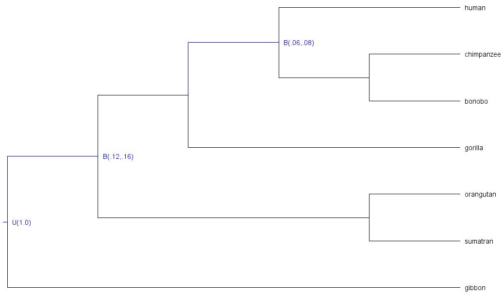
As you can see, the following nodes were calibrated:
- t_n8: root age, constrained with upper bound U(1.0) (maximum age = 1.0; time unit = 100MY | 100MY )
- t_n9: last common ancestor of great apes (all taxa but gibbon), node constrained with soft bound B(.12,.16) (minimum age = .12, maximum age = .16; time unit = 100MY | 12MY - 16MY)
- t_n11: last common ancestor of human, chimpanzee, and bonobo; node constrained with soft bound B(.06,.08) (minimum age = .06, maximum age = .08; time unit = 100MY | 8MY).
We can run MCMCtree without data (e.g., four independent chains) to check whether the samples collected for each chain are indeed sampling from the prior (target distribution) and will within our expectations based on calibration densities we specified.

Marginal densities VS calibration densities of those nodes which ages were constrained

While the plots above are very informative, they do not really show what densities the uncalibrated nodes have, and thus it is hard to understand whether they have been misspecified. In order to plot all marginal densities (not only those from the calibrated nodes) we can use Tracer, R, or any other tool you prefer to better understand how the joint prior on divergence times looks like:

Marginal densities for all node ages (calibrated and uncalibrated)

In this case, it seems that there are no problematic chains and all densities fall within the expected ages based on the age constraints specified for 2 internal nodes and the root.

Note

Given that all the chains seem to have converged to the same target distribution (prior), we could also combine the samples collected by all chains as a unique larger sample. Note that we could also run other MCMC diagnostics to make sure that the chains are "healthy" such as convergence plots or calculate statistics such as Rhat, ESS, tail-ESS, bulk-ESS, etc.

Warning

The component $f(t_{C})$ appears twice in Eq. (2) which, as acknowledge by Heled and Drummond (2019), does not follow the rules of probability calculus:

"If the birth rate and the calibration density are really independent sources of information about the phylogeny, then this may not be a bad method to construct the calibrated tree prior, although **this construction certainly does not follow the rules of probability calculus**. Specifically, the multiplicative construction is problematic in situations where the researcher expects the calibration prior to represent the marginal distribution of the calibrated node, and can lead to unexpected result."

The duplicated term $f(t_{C})$ will be altered by truncation, but the effect on estimated divergence times may not be too strong.

In addition, dos Reis (2016) pointed out that the conditional prior $f_{BD}(t_{C}|t_{1})$ of Yang and Rannala (2006); see Eq. (1) above is misspecified because labelled histories are not distinguished from rooted trees when calculating this term. Ordered times and labelled times are different random variables, and so one should not expect them to have the same probability distribution see section 4 in dos Reis (2016) for technical details, which results in a misspecified marginal density.

In essence, both the conditional and the multiplicative constructions are incorrect, but the algorithm proposed by dos Reis (2016), which does follow the rules of probability calculus, has not yet been implemented in any dating program.

Important

It is noteworthy that the density for calibrated nodes is affected by truncation in both the multiplicative and the conditional approaches. As shown in Barba-Montoya 2018, the conditional construction leads to marginal priors (i.e., "effective priors") that are closest to the original calibration densities (i.e., "user-specified priors") when truncation is minimal. When truncation is severe, effective priors will differ substantially from the user-specified priors regardless of the approach. Nevertheless, while the density for non-calibrated nodes is affected by the aforementioned mistake in the conditional construction, the multiplicative construction is not. On balance, we recommend that the multiplicative approach be used in such cases (as it generates more reasonable densities for non-calibration nodes) and that users check and confirm that the marginal densities for the "effective priors" (after the program has applied the truncation) are biologically reasonable. Consequently, running the program without data to check whether the marginal densities are reasonable must be done before analysing the data, regardless of using the conditional or the multiplicative construction. If some of those priors look biologically unrealistic, users should adjust the calibration densities in the tree file, re-run the program, and check again. This advice would not only apply to MCMCtree, but also to any other Bayesian dating program that can be used for timetree inference.

kappa_gamma: this variable specifies the shape ($\alpha$) and scale ($\beta$) parameters in the gamma prior for parameter $\kappa$ (i.e., the transition/transversion rate ratio) in models such as K80 and HKY85. Please note that this variable has no effect in models such as JC69, which does not have the parameter. Note that the mean of a gamma distribution with parameters $\alpha$ and $\beta$ can be calculated as $\alpha/\beta$, and the variance as $\alpha/\beta^2$. Please note that these variables are only enabled when usedata = 1 (i.e., exact likelihood calculation) and have no effect when usedata = 2 <inBV> (i.e., approximate likelihood calculation), in which case there is no need to include this prior in the control file (i.e., the in.BV file contains the branch lengths, the gradient, and the Hessian estimated under a substitution model that will have accounted for this prior if $\alpha$ is a model parameter; otherwise this setting is ignored).
alpha_gamma: this variable specifies the shape ($\alpha$) and scale ($\beta$) parameters in the gamma prior for the shape parameter for gamma rates among sites in models such as JC69$+\Gamma$, K80$+\Gamma$, etc. The gamma model of rate variation is assumed only if the variable alpha is assigned a positive value. Please note that these variables are only enabled when usedata = 1 (exact likelihood calculation) and have no effect when usedata = 2 <inBV> (approximate likelihood calculation), in which case there is no need to include this prior in the control file (i.e., the in.BV file contains the branch lengths, the gradient, and the Hessian estimated under a substitution model that will have accounted for this prior if $\alpha$ is a model parameter; otherwise this setting is ignored).
rgene_gamma: this variable specifies the parameters in the prior for the locus rates $\mu_{i}$. Two priors are implemented for locus rates ($\mu_{i}$), as summarised in Zhu et al. (2015). They can be specified by using the following options:
```
rgene_gamma = au bu a prior
```
- [DEFAULT] Gamma-Dirichlet prior (dos Reis et al. 2014): parameter au is $\alpha_{\mu}$, bu is $\beta_{\mu}$, and a is $\alpha$ in Eqs. 3-5 in the aforementioned paper. Option prior should be set to 0, but this is already the default option.
- Conditional i.i.d. prior (Zhu et al. 2015): au, bu, and a are the same parameters as per the gamma-Dirichlet prior, which are defined in Eq. 8 in the aforementiond paper. One can enable the conditional i.i.d. prior by setting the fourth option for rgene_gamma (the type of prior) to 1.
The gamma-Dirichlet and conditional i.i.d. priors are expected to be similar especially if the number of genes or loci or partitions is large. In the implementation, $\bar{\mu}$ is a parameter in the conditional i.i.d. prior but not in the gamma-Dirichlet prior. The prior on $\sigma_{i}^2$ (variable sigma2_gamma) has parameters au ($\alpha_{\mu}$), bu ( $\beta_{\mu}$), a ($\alpha$) specified in the same way as rgene_gamma, and so the same form of prior (either the gamma-Dirichlet or the conditional i.i.d.) is used for both $\mu_{i}$ and $\sigma_{i}^2$.

For instance, given that the default value of $\alpha = 1$ and the default prior is the gamma-Dirichlet prior (fourth option is set to $0$), the following pair of settings for rgene_gamma and sigma2_gamma are equivalent:
```
* Specifying alpha and the type of prior, despite these values
* being the default ones
rgene_gamma = 100 1000 1.0 0
sigma2_gamma = 4 100 1.0

* Using default settings (alpha=1 and prior=0), no need to
* specify these parameter values in the control file if
* they are the same
rgene_gamma = 100 1000
sigma2_gamma = 4 100
```
To specify the conditional i.i.d. prior, all the parameter values would need to be included:
```
rgene_gamma = 100 1000 1.0 1
sigma2_gamma = 4 100 1.0
```

Important

Under the global-clock model (clock = 1), the independent-rates log-normal relaxed-clock model (clock = 2), and the autocorrelated-rates relaxed-clock model (clock = 3), $\mu_{i}$ is the overall rate for locus $i$. In the example above, $\mu_{i}$ has the prior mean $\alpha_{\mu}/\beta_{\mu}=100/1000 = 0.1$, that is, one change per site per time unit. If one time unit is 100MY, this means an overall average rate of $10^{–9}$ substitutions per site per year. The variance in the logarithm of the rates ($\sigma_{i}^2=100/1000^2 = 0.01$ in the example above) of this gamma prior specifies how confident you are about the overall rate. The third parameter $\alpha$ ($\alpha = 1$ in the example above) specifies how variable the overall rates are among loci. This parameter has more or less the same interpretation as the shape parameter $\alpha$ for the gamma model of variable rates among sites (Yang 1993), with a large $\alpha$ (say, $\alpha\approx 100$) meaning nearly identical rates among loci and small values (e.g., $\alpha=1$ or $\alpha=0.5$) highly variable rates among loci.
You must adjust this prior to suit your data and the chosen time scale. DO NOT use the default settings that you may find in template control files or control files used in other analyses.

If you do not have information about the overall rate, please check the recommendations given in the Overview section of this site to derive a rough rate estimate (for use as the prior mean) and adjust the parameter values of the rate prior (rgene_gamma) and the prior on $\sigma_{i}^2$ (sigma2_gamma).

sigma2_gamma: this variable specifies the shape and scale parameters in the conditional i.i.d. or gamma-Dirichlet prior for parameter $\sigma_{i}^2$ as explained in paragraph above under rgene_gamma. Note that $\sigma_{i}^2$ specifies how variable the rates are across branches or how seriously the clock is violated at the locus. This prior is enabled only when one of the two relaxed-clock models are specified (i..e, clock = 2 or clock = 3), with a larger $\sigma_{i}^2$ indicating more variable rates (Rannala and Yang 2007). In other words, if clock = 1 (strict clock model), this prior has no effect.

In the independent-rates log-normal relaxed-clock model (clock = 2), rates for branches are independent variables from a log-normal distribution (Rannala and Yang 2007, see equation 9),

$$f(r|\mu,\sigma^{2})=\frac{1}{r\sqrt{2\pi\sigma^{2}}}exp( -\frac{1}{2\sigma^{2}}[log(r/\mu)+\frac{1}{2}\sigma^{2}]^{2} ) ,0<r<\infty$$

Eq. (3)

with mean $E(r)=\mu$ and variance $Var(r)=(e^{\sigma^{2}}-1)\mu^{2}$. The distribution is completely specified by $\mu$ and $\sigma^2$. Parameter $\sigma^2$ is the variance of $log(r)$.

The autocorrelated-rates relaxed-clock model (clock = 3) specifies the density of the current rate $r$ given that the ancestral rate time $t$ ago is $r_{A}$. Following Eq. 2 in Rannala and Yang 2007:

$$f(r|r_{A},t\sigma^{2})=\frac{1}{r\sqrt{2\pi t\sigma^{2}}}exp( -\frac{1}{2t\sigma^{2}}[log(r/r_{A})+\frac{1}{2}t\sigma^{2}]^{2}) ,0<r<\infty$$

Eq. (4)

with mean $E(r)=r_{A}$ and variance $Var(r)=(e^{t\sigma^{2}}-1)r^2_{A}$. Note that parameter $\sigma^2$ in Eq. (4) above is equivalent to $v$ in Kishino et al. (2001).

Important

What happens when we change the time unit?

When clock = 2:
Let us write $t$ for time. If we change the time scale by a constant factor so that the new time is $t_{scaled} = kt$, then the substitution rate needs to be re-scaled accordingly so that the new rate is $r_{scaled} = r/k$. For a constant $a$, $E(aX) = aE(X)$ and $Var(aX) = a^2Var(X)$. Therefore, the rate $r_{scaled}$ in the transformed time scale has mean

$E(r_{scaled})=E(r/k)=\frac{1}{k}E(r)=\frac{\mu}{k}$

and variance

$Var(r_{scaled})=Var(r/k)=\frac{1}{k^{2}}Var(r)=\frac{1}{k^{2}}(e^{\sigma^{2}}-1)\mu^{2}=(e^{\sigma^{2}}-1)(\frac{\mu}{k})^{2}$.

Here, $r$ is log-normally distribute with parameters $\sigma^2$ and $\mu_{scaled}=\mu/k$. When changing the time scale, we need to change the rate prior accordingly. If $\mu$ has a gamma prior $f(\mu)=Gamma(\mu|\alpha,\beta)$, then $\mu_{scaled}$ must have the equivalent gamma prior $f(\mu_{scaled})=Gamma(\mu_{scaled}|\alpha,k\beta)$. Nevertheless, $\sigma^2$ is unchanged during the scale transformations, and thus the prior on $sigma^2$ (sigma2_gamma) must remain unchanged. The birth and death rates in the birth-death process with species sampling (but not the sampling fraction!) need to be changed too. E.g.: if we change the time scale from 100MY to 1MY (i.e., $t_{scaled}=100t$ and $r_{scaled}=r/100$), we would need to change the node age constraints included in the tree file (e.g., from B(6,8) to B(0.06,0.08)), the birth and death rates of BDparas in the control file (e.g., from BDparas = 1 1 0.1 to BDparas = 0.01 0.01 0.1) and the scale parameter of rgene_gamma in the control file (e.g., from rgene_gamma = 2 20 to rgene_gamma = 2 2000).
When clock = 3:
Under the autocorrelated-rates relaxed-clock model, the rate follows a log-normal distribution with parameters $\mu$ and $t\sigma^2$. Now, the variance of $log(r)$ is a function of the time $t$. Given that we are changing the time scale, the new variance is $t_{scaled}\sigma_{scaled}^2$, where $\sigma_{scaled}^2=\sigma^2/k$. Given that the prior on $\sigma^2$ is $Gamma(\sigma^2|\alpha,\beta)$, then for $\sigma_{scaled}^2$ is $Gamma(\sigma_{scaled}^2|\alpha,k\beta)$. Consequently, if we change the time scale when analysing our data under the autocorrelated-rates relaxed-clock model, we will need to change the scale parameter of sigma2_gamma in the control file too (e.g., sigma2_gamma = 1 10 to sigma2_gamma = 1 1000).

Running the analysis with the new time scale will lead to the same results as the previous analysis you ran, but you will see that all posterior divergence times and rates are scaled accordingly by constant $k$.

[NOTE]: the notation used above has been adapted to make it easier to write down what happens when we change the time unit. Remember that the notation for locus rates is $\mu_{i}$ and $\sigma_{i}^2$ for the variance in the logarithm of the rate in dos Reis et al. (2014) and Zhu et al. (2015).

print: there are various options that can be enabled when using this variable. To summarise the samples collected during the MCMC and write them in the output file specified in variable mcmcfile, option print = 1 should be used (default option). To test the program and just print the posterior means on the screen, you may use print = 0. When enabling relaxed-clock models (i.e., clock = 2 or clock = 3), you may want to print the rates for branches for each locus (i.e., for each "alignment block" or "partition" in the input sequence file), which can be done by setting option print = 2. If you ran an analysis but the MCMC did not finish, you may not obtain the output tree file with divergence times (i.e., FigTree.tre file). In such a case, you may want to use option print = -1 so that you can summarise the samples that have already been collected by the unfinished runs and map them onto the fixed tree topology. You will need to specify the output file with MCMC samples in variable mcmcfile (the samples to be summarised will be read from this file), the calibrated fixed tree topology with variable treefile (the mean divergence times and confidence intervals will be mapped onto this topology). While the sequence data are not used when print = -1, you must also specify an alignment file with variable seqfile so that MCMCtree checks that there are no missing taxa and that the same tag identifiers have been used in both the alignment and tree files.

Note

If you run print = -1, you may want to create a new folder with the input files (sequence file, tree file, output file from your unfinished analysis with all MCMC samples) and reuse the control file but now change variable print to print = -1. If you have a large molecular alignment and would like to reduce the time MCMCtree takes to read your input sequence file, you may use a dummy alignment instead (i.e., one line for each taxon present in the phylogeny and 2 characters, thus the PHYLIP header shall be <num_taxa> 2).

burnin, sampfreq, nsample: the program will discard the samples collected during the burn-in phase (burnin), and thus the output file with MCMC samples (i.e., output files specified with variable mcmcfile) will never store those samples. You need to use variable sampfreq to increase or decrease the frequency with which samples are being saved in the output MCMC file. The total number of samples that you would like to collect in your output MCMC file is controlled with variable nsample. The total number of iterations can be calculated as burnin + sampfreq x nsample.

Important

To avoid large output MCMC files, it is recommended that you collect between 10,000 to 20,000 samples so that your disk space is not compromised (Nascimento et al. 2017). You can increase the number of iterations by increasing the sampling frequency instead while keeping the same number of samples.

checkpoint: this variable will take three options: the type of checkpointing enabled (1: "save" mode and 2: "resume" mode), the probability that will indicate how often MCMCtree will write into the checkpoint file, and the name of the checkpoint file (e.g.,if no third option is provided, a default name in the form of mcmctree.ckpt1 will be used). To enable checkpointing for the first run, the first option of variable checkpoint needs to be 1 ("save" mode). Please note that the implemented checkpointing feature does not save the memory image in the usual sense of the word. Instead, MCMCtree will save the current state of the Markov chain (e.g., divergence times, rates for loci, step lengths) in a file (e.g., the default name is mcmctree.ckpt, but you can modify this name via the third option for variable checkpoint).

The conditional probability vectors will not be saved; they are recalculated when the run is resumed. For instance, a run may have ended abruptly or more samples may be required as the chain may have not reached convergence, thus the analysis needs to be resumed from the last state saved in the checkpoint file generated from the first run. To enable the "resume" mode, a new analysis should be carried out with the first option of the variable checkpoint now set to 2. When this option is enabled, the program will read the control file and input sequence file, allocate enough memory accordingly, and then fix the state of the Markov chain by reading the checkpoint file (e.g., mcmctree.ckpt, mcmctree.ckpt1, or any other name you have given to the file using the third option), which will have the last saved state of the chain. Lastly, the MCMC will restart from that point by internally setting burnin = 0. In essence, MCMCtree uses the last saved parameter values and sets them as initial values, without running the burn-in phase. MCMCtree will then collect as many samples as those specified via variable nsample with a sampling frequency as specified in variable sampfreq in the control file that has just been read.

Lastly, the second option is a probability that specifies how often MCMCtree will save the state of the Markov chain into the checkpoint file. For instance, prob = 0.01 means that, if the run is not interrupted, MCMCtree will be saving 100 times the state of the Markov chain into the checkpoint file. As aforementioned, output files are re-written, and so will the checkpoint file. Please follow the guidance given above to avoid losing important output files due to overwriting.

Warning

Please note that output files are always overwritten when you re-run the analysis in the same folder. For instance, the output MCMC file from the first run when checkpoint was set to mode "save" (first option set to 1) will be destroyed and a new one will be generated; the same would apply to the other output files. To avoid losing such important files (e.g., you do not want to lose the output MCMC file with all the samples that you have been collected so far!), you may want to save the output files from the first run somewhere safe in your file system before re-running the analysis with the "resume" mode (in case you are re-running everything under the same folder). Alternatively, you may want to create a new folder where you run the analysis with variable checkpoint set to "resume" mode (2). The latter option will allow you to keep your original folder untouched while the "resume" analysis would take place elsewhere (no danger to overwrite the files output during the first run!).

Important

At the end of your analysis, you will need to combine the samples collected during the first run and those collected in subsequently resumed runs (e.g., you may have as many output MCMC files as times you have had to resume the run with checkpoint = 2 <prob> <checkpoint_fname>). You can create a unique output MCMC file with all the samples that have been collected throughout the various "resumed" runs for that specific chain. You can either do this manually using a text editor or write a script that can do this.

Important

You could use the checkpoint files with the latest states saved to restart multiple MCMC runs at the same time. For instance, if your run has failed but you enabled the save mode with the first option being 1, you will have the output checkpoint file. You could copy this file into different folders, set variable seed = -1 in the corresponding control files, and resume the chain multiple times independently. While the initial state is the same, the samples collected by the independent runs will all be different because of the different random number used as per variable seed = -1.

duplication: this variable is a switch (0 for no and 1 for yes) to turn on the option for duplicated genes/proteins. There are two types of constraints that can be enabled, equality and inequality constraints, which will be triggered based on the notation used in the tree file to identify specific nodes. For instance, when using paralogous genes, there may be some nodes in the tree that correspond to the same speciation event, which we may want to fix to the same age. We can identify such nodes in the tree file by using node labels such as #1, #2, etc. The following Newick trees show how this notation would be incorporated to specify this type of node age constraints in MCMCtree:
```
(((A1, A2) [#1 B{0.2, 0.4}], A3) #2, ((B1, B2) #1, B3) #2 ) 'B(0.9,1.1)';
(((A1, A2) [#1 B{0.2, 0.4}], A3) #2, ((B1, B2) [#1], B3) [#2] ) 'B(0.9,1.1)';
(((A1, A2) [#1 B{0.2, 0.4}], A3) #2, ((B1, B2) [#1 B{0.2, 0.4}], B3) #2 ) 'B(0.9,1.1)';

(((A1, A2) [#1 >0.2 <0.4], A3) #2, ((B1, B2) #1, B3) #2 ) >0.9<1.1;
(((A1, A2) [#1 >0.2 <0.4], A3) #2, ((B1, B2) [#1], B3) [#2] ) >0.9<1.1;
(((A1, A2) [#1 >0.2 <0.4], A3) #2, ((B1, B2) [#1 >0.2 <0.4], B3) #2 ) >0.9<1.1;
```
All the trees above are equivalent ways of specifying equality constraints (also known as cross-bracing) in MCMCtree, which could be displayed as shown below in Figure 1a:

Figure 1: (a) a tree with labelled nodes to apply equality constraints. By labelling nodes $a$ and $b$ using the same label #1, and nodes $u$ and $v$ using the same label #2, the duplication option can be used to enforce equality constraints on node ages: $t_{a} = t_{b}$, $t_{u} = t_{v}$. Black dots indicate nodes with calibrations. (b) The duplication option can also be used together with a ghost species to enforce inequality constraints on node ages (e.g., $t_{u} > t_{v}$). The ghost species appears in the tree, but not in the data file as there is no data for it. Since node $g$ (the ancestor for the ghost species) is ancestral to an older than node $v$ ($t_{g} > t_{v}$) the equality constraint $t_{u} = t_{g}$ means that $t_{u} > t_{v}$.

In the examples shown in Fig 1a, $A$ and $B$ are paralogs, while $A_{1}$, $A_{2}$, and $A_{3}$ are different species of $A$ and $B_{1}$, $B_{2}$, and $B_{3}$ are different species of $B$. Node $r$ represents a duplication event while other nodes are speciation events. Node $a$ (the $A_{1}-A_{2}$ ancestor) and node $b$ (the $B_{1}-B_{2}$ ancestor) are assigned the same label (#1), so that they share the same age: $t_{a} = t_{b}$. In other words, nodes $a$ and $b$ are cross-braced. Similarly node $u$ and node $v$ have the same age: $t_{u} = t_{v}$. In addition, there is another node age constraint based on fossil evidence to further constrain the age of nodes $a$ and $b$: $0.2 < t_{a} = t_{b} < 0.4$, equivalent to the traditional MCMCtree notations 'B(0.2,0.4)' or '>0.2<0.4'. There is another calibration on the root: $< 0.9 < t_{r} < 1.1$, equivalent to the traditional MCMCtree notations 'B(0.9,1.1)' or '>0.9<1.1'.

Among the nodes on the tree with the same label, one is chosen as the "driver" node while the others are labelled as "mirror" nodes. If calibration information is provided on one of the shared nodes, the same information will therefore apply to all shared nodes. If calibration information is provided on multiple shared nodes, that information must be the same. The time prior (or the prior on all node ages on the tree) is constructed by using a density at the root of the tree (specified by the user via the input tree file), while the ages of all non-calibration nodes are given by the uniform density. This time prior is similar to that used by Thorne et al. (1998). The parameters in the birth-death process with species sampling (i.e., $\lambda$, $\mu$, $\rho$; which are specified using variable BDparas) are ignored.

This variable can also be used to specify inequality constraints (see Fig. 1b above). To constrain node $u$ to be older than node $v$ ($t_{u} > t_{v}$), we have to include a "ghost species" in the tree, creating a new node $g$ that is ancestral to node $v$. By constraining node $g$ to have the same age as node $u$ (i.e., they are both identified with label #2), we enforce the inequality constraint $t_{u} > t_{g}$.

The different notations that can be used to specify the inequality constraints shown in Figure 1b are as follows:
```
(((A1, A2) [#1 B{0.2, 0.4}], A3) #2, (((B1, B2) #1, B3), ghost) #2 ) 'B(0.9,1.1)';
(((A1, A2) [#1 B{0.2, 0.4}], A3) #2, (((B1, B2) [#1], B3), ghost) [#2] ) 'B(0.9,1.1)';
(((A1, A2) [#1 B{0.2, 0.4}], A3) #2, (((B1, B2) [#1 B{0.2, 0.4}], B3), ghost) #2 ) 'B(0.9,1.1)';

(((A1, A2) [#1 >0.2 <0.4], A3) #2, (((B1, B2) #1, B3), ghost) #2 ) >0.9<1.1;
(((A1, A2) [#1 >0.2 <0.4], A3) #2, (((B1, B2) [#1], B3), ghost) [#2] ) >0.9<1.1;
(((A1, A2) [#1 >0.2 <0.4], A3) #2, (((B1, B2) [#1 >0.2 <0.4], B3), ghost) #2 ) >0.9<1.1;
```
A lateral gene transfer (LGT) event is one of the main possible scenarios for inequality constraints to be enabled. In the example above, branch $u$ would be the donor and branch $v$ would be the recipient, which results in node $u$ being older than node $v$.

Important

More than two nodes can have the same label, but one node cannot have two or more labels. In addition, the rate prior does not distinguish between speciation and duplication events.

Important

Please note that the ghost species $g$ does not appear in the sequence data file as there is no data available for it; it is only include in the input tree file to create a new node ($g$) that has the same age as node $u$ but that, at the same time, is older than $v$. In other words, the input sequence file does not need to be modified nor include any sequence for this ghost lineage. Only the input tree file is to be modified to incorporate this ghost lineage.

Important

There is no information about the precise time of the LGT event. The inequality constraints merely specify the relative order of the ages of two nodes on the tree, with the donor species being older than the recipient.

Older variables

The variables below were implemented in older PAML versions. While the analyses with the latest PAML version will not be compromised by including these variables in the control file, it is recommended to avoid using them:

finetune (deprecated): this variable is currently deprecated as MCMCtree automatically auto-tunes the step lengths used in the proposals in the MCMC algorithm. Therefore, if you include this setting in the control file, you will see the following message printed on the screen output: finetune is deprecated now.. Nevertheless, you can find below the settings of this variable for the record.
In the control file, the options for variable finetune could look like the following:
```
finetune = 0: 0.04 0.2 0.3 0.1 0.3 * auto (0 or 1) : times, musigma2, rates, mixing, paras,
finetune = 1: .05 .05 .05 .05 .05 .05 * auto (0 or 1) : times, musigma2, rates, mixing, paras,
```
The first value before the colon (i.e., either 0 or 1) is a switch, with 0 meaning no automatic adjustments by the program and 1 meaning automatic adjustments by the program. Following the colon, you shall find the step lengths for the proposals used in the program. The proposals are as follows: (a) to change the divergence times, (b) to change $\mu_{i}$ (and $\sigma_{i}^2$ if clock = 2 or clock = 3), (c) to change the rate for loci for the relaxed clock models, (d) to perform the mixing step (see page 225 in Yang and Rannala 2006), and (e) to change parameters in the substitution model (such as $\kappa$ and $\alpha$ in HKY+G). If you choose to let the program adjust the step lengths, the burnin variable has to be >200 and then the step lengths specified via finetune will be the initial step lengths. Consequently, the program will try to adjust these values by using the information collected during the burn-in phase (as many iterations as specified wih variable burnin).The program will do this action twice, once at half of the burn-in and another time at the end of the burn-in.
The following notes are for manually adjusting the step lengths. You can use them to generate good initial step lengths as well for the option of automatic step length adjustment.

A few seconds or minutes (hopefully not hours) after you start the program, the screen output will look like the following:
```
-20% 0.33 0.01 0.25 0.00 0.00 1.022 0.752 0.252 0.458 0.133 0.843 - 0.074 0.787 -95294.7
-15% 0.33 0.01 0.25 0.00 0.00 1.021 0.751 0.253 0.457 0.130 0.841 - 0.067 0.783 -95295.4
-10% 0.33 0.00 0.26 0.00 0.00 1.022 0.752 0.254 0.458 0.129 0.842 - 0.065 0.781 -95294.6
-5% 0.33 0.00 0.25 0.00 0.00 1.022 0.751 0.254 0.457 0.128 0.841 - 0.063 0.780 -95292.4
0% 0.32 0.00 0.25 0.00 0.00 1.022 0.751 0.254 0.457 0.128 0.841 - 0.063 0.780 -95290.2
2% 0.32 0.00 0.27 0.00 0.00 1.014 0.746 0.253 0.453 0.126 0.833 - 0.059 0.784 -95290.4
```
The output that you see above is generated from a run under the JC model and global clock (clock = 1). The percentage % (first value) indicates the progress of the run, with negative values for the burn-in. Then, the five proportions (e.g., 0.33 0.01 0.25 0.00 0.00 on the first line) are the acceptance proportions (Pjump) for the corresponding proposals. The optimal acceptance proportions are around 0.3, and you should try to make them fall in the interval (0.2, 0.4) or at least (0.15, 0.7). If the acceptance proportion is too small (say, <0.10), you decrease the corresponding finetune parameter. If the acceptance proportion is too large (say, >0.80), you increase the corresponding finetune parameter. In the example here, the second acceptance proportion, at 0.01 or 0.00, is too small, so you should stop the program (i.e., press Ctrl-C on your keyboard; you are supposed to run this test before you run this analysis!) and modify the control file to decrease the corresponding finetune parameter (change 0.2 into 0.02, for example). Then run the program again, observe it for a few seconds or minutes and then kill it again if the proportions are still not good. Repeat this process a few times until every acceptance proportion is reasonable. This is not quite so tedious as it may sound, and it is worth doing so that the chain samples from the correct area of the parameter space (the target distribution).

The finetune parameters in the control file are in a fixed order and always read by the program even if the concerned proposal is not used (in which case the corresponding finetune parameter has no effect). In the above example, JC does not involve any substitution parameters, so that the 4th finetune parameter has no effect, and the corresponding acceptance proportion is always 0. This proportion is always 0 also when the approximate likelihood calculation is used (usedata = 2 <inBV>) because, in such a case, the likelihood is calculated by fitting the branch lengths to a normal density, ignoring all substitution parameters like $\kappa$, $\alpha$, etc. If clock = 1, there are no parameters in the rate-drift model, so that the 5th acceptance proportion is always 0. Note that the impact of the finetune parameters is on the efficiency of the algorithm, or on how precise the results are when the chain is run for a fixed length. Even if the acceptance proportions are too high or too low, reliable results will be obtained in theory if the chain is run sufficiently long. This effect is different from the effect of the prior, which affects the posterior estimates.

Calibrations: how to set up node age constraints?

Node age constraints based on fossil evidence are specified in the input tree file in the form of statistical distributions of divergence times (or node ages in the fixed tree topology). To see a list of the statistical distributions implemented in MCMCtree that you can use to constrain node ages, please see the table below (Table 1).

In this section, “fossil” means any kind of external calibration data, including geological events. For a sensible analysis, one should have at least one lower bound and at least one upper bound on the tree, even though they may not be on the same node.

Important

The gamma, skew-normal, and skew-t distributions can act as both bounds, so one such calibration is enough to anchor the tree to enable a sensible analysis.

Table 1. Calibration distributions.

Calibration	#p	Specification	Density
L (lower or minimum bound)	4	`'>0.06'` or `'L(0.06)'` or `'L(0.06,0.2)'` or `'L(0.06,0.1,0.5)'` or `'L(0.06,0.1,0.5,0.025)'`	`'L(tL, p, c, pL)'` specifies the minimum-age bound `tL`, with offset `p`, and scale parameter `c`, and tail probability for the lower bound `pL`. The default values are `p = 0.1`, `c = 1`, and pL = 0.025, so `'>0.06'` (or `'L(0.06)'`) means `'L(0.06, 0.1, 1, 0.025)'`, while `'L(0.06, 0.2)'` means `'L(0.06, 0.2, 1, 0.025)'`. If you would like the minimum bound to be hard, please use `pL = 1e-300`, but do not use `pL = 0`. In other words, use `'L(0.06, 0.2, 1, 1e-300)'`, not `'L(0.06, 0.2, 1, 0)'`.
U (upper or maximum bound)	2	`'>0.08'` or `'L(0.08)'` or `'L(0.08,0.025)'`	See Eq. 16 and Fig. 2b in Yang and Rannala (2006). `'U(tU, pU)'` specifies the maximum-age bound `tU`, with upper tail probability `pU`. The default value is `pU = 0.025`, so `'<0.08'` (or `'U(0.08)'`) means `'U(0.08, 0.025)'`. For example, `'U(0.08, 0.1)'` means that there is 10% probability that the maximum bound 8MY is violated (i.e., the true age is older than 8MY).
B (lower & upper bound or minimum & maximum bound)	4	`'>0.06<0.08'` or `'L(0.08)'` or `'L(0.08,0.025)'`	See Eq. 17 and Fig. 2c in Yang and Rannala (2006). `'B(tL, tU, pL, pU)'` specifies a pair bound, so that the true age is between `tL` and `tU`, with the lower and upper tail probabilities to be `pL` and `pU`, respectively. The default values are `pL = pU = 0.025`.
G (Gamma)	2	`'G(alpha,beta)'`	See Eq. 18 and Fig. 2d in Yang and Rannala (2006).
SN (skew normal)	3	`'SN(location, scale, shape)'`	See Eqs. 5-8 and corresponding plots below.
ST (skew-t)	4	`'SN(location, scale, shape, df)'`	See Eqs. 9-13 and corresponding plots below.
S2N (skew 2 normals)	7	`'SN2(p1, loc1, scale1, shape1, loc2, scale2, shape2)'`	p₁=1-p₁ mixture of two skew normals.

Note: #p is the umber of parameters in the distribution to be supplied by the used.

Below, you can find a summary explaining the different types of calibration densities implemented in MCMCtree:

Lower bound (minimum age): this calibration density is specified as '>tL', 'L(tL,p)', 'L(tL,p,c)'. or 'L(tL, p, c, pL)'. E.g., 'L(0.06)' means that the node age is at least 6MY, assuming that one time unit is 100 million years.
Since PAML version 4.2, the implementation of the minimum bound has changed. Instead of the improper soft flat density of Figure 2a in Yang and Rannala (2006), a heavy-tailed density based on a truncated Cauchy distribution is now used (Inoue et al. 2010). The Cauchy distribution with location parameter $t_{L}(1 + p)$ and scale parameter $ct_{L}$ is truncated at $t_{L}$, and then made soft by adding $\alpha_{L} = 2.5%$ of density mass left of $t_{L}$. The resulting distribution has mode at $t_{L}(1 + p)$. The $\alpha_{L} = 2.5%$ limit is at $t_{L}$ and the 97.5% limit is at

$t_{97.5\%}=t_{L}[1+p+c\times cot(\frac{\pi A\alpha_{R}}{1-\alpha_{L}})]$,

where $\alpha_{R}=1-0.975$ and $A=\frac{1}{2}+\frac{1}{\pi}tan^{-1}(\frac{p}{c})$. This is slightly more general than the formula in the paragraph below equation (26) in Inoue et al. (2010), in that $\alpha_{L}$ and $\alpha_{R}$ are arbitrary: to get the 99% limit when $t_{L}$ is a hard minimum bound, use $\alpha_{L} = 0$ and $\alpha_{R} = 0.01$ so that $t_{99\%}=t_{L}[1+p+c\times cot(0.01\pi A)]$.

If the minimum bound $t_{L}$ is based on good fossil data, the true time of divergence may be close to the minimum bound, so that a small $p$ and small $c$ should be used. It is noted that $c$ has a greater impact than $p$ on posterior time estimation. The program uses the default values $p = 0.1$ and $c = 1$, unless users set different parameter values using the notation described above. Please note that you should use different values of $p$ and $c$ for each minimum bound based on a careful assessment of the fossil evidence on which the bound is based.

Below, you can find the R code to generate two different plots in which parameter values $p$ and $c$ are changed. The minimum bound is fixed at $t_{L} = 1$, but one time unit can mean anything like 100MY or 1000MY. For each value of $p$ ($0.1$ and $0.5$), the four curves correspond to $c = {0.2, 0.5, 1, 2}$ (from top to bottom near the peak). The 2.5% limit is at 1, while the 97.5% limits for those values of $c$ are $4.93$, $12.12$, $24.43$, $49.20$, respectively, when $p = 0.1$. When $p = 0.5$, then these values are $4.32$, $9.77$, $20.65$, $44.43$ (please note that those values were incorrectly calculated in Inoue et al. (2010)).
```
  par( mfrow = c( 1, 2 ) )
  cols <- c(  "#000000","#D55E00", "#023903", "#56B4E9", "#CC79A7")
  count <- 0
  for( j in c( 0.1, 0.5 ) ){
    for( i in c( 0.2, 0.5, 1, 2 ) ){
      count <- count + 1
      if( count == 1 ){
        curve( mcmc3r::dL( x, tL = 1, p = j, c = i, pL = 0.025 ),
              from = 0.8, to = 2, n = 1e4, xlim = rev( c( 0.8, 2 ) ),
              xlab = "Time (Mya)", ylab = "Density",
              main = paste( "Lower minimum | p = ", j, sep = "" ),
              col = cols[count] )
      }else{
        curve( mcmc3r::dL( x, tL = 1, p = j, c = i, pL = 0.025 ),
              col = cols[count], add = TRUE )
      }
    }
    legend( "topleft",  lty = 1, col = cols,
            legend = c( "c = 0.2", "c = 0.5", "c = 0.1", "c = 2" ) )
    count <- 0
  }
```

Upper bound (maximum age): this calibration density is specified as '<tU' or 'U(tU)'. For instance, 'U(0.08) would mean that the node age is at most 8MY (time unit = 100MY).
Lower and upper bounds (minimum and maximum ages): this calibration density is specified as '>tL<tU', 'B(tL,tU)', 'B(tL,tU,pL,pU)'. For instance, if we were to specify a minimum age of 6MY and a maximum age of 8MY, we could use 'B(6,8)' of both bounds were soft (i.e., pL = pU = 0.025). If we were to use different tail probabilities or hard bounds, we would need to use the long notation. E.g.: 'B(6,8,1e-300,1e-300)' would enforce soft minimum and maximum bounds.
Gamma distribution: this calibration density is specified as 'G(alpha,beta)', and thus users must specify the values of shape parameter $\alpha$ and scale parameter $\beta$. The mean of the distribution is $\alpha/\beta$, which would be the expected mean estimated time for the node which age is being constrained. For instance, for a very narrow density around 0.07 (7MY, time unit = 100MY), we could choose a large value of $\alpha$ such as $\alpha=188$. To calculate $\beta$, we can do the following: $\beta= 188/0.07 \approx 2686$. If we want a more diffuse gamma distribution, we can choose smaller values of $\alpha$. Below, you have the R code with which different distributions with mean 0.07 are drawn which are eiter narrower or more diffuse to reflect your certainty on such an estimated value. Below, you can find an example R code to plot various Gamma densities with different shapes based on smaller and larger values of $\alpha$:
```
cols <- c(  "#000000","#D55E00", "#023903", "#56B4E9", "#CC79A7")
mean_t <- 0.07
alpha  <- c( 188, 100, 50, 10, 2 )
beta   <- alpha/mean_t
for( i in seq(1, length(alpha) ) ){
  if( i == 1 ){
    curve( dgamma( x, alpha[i], beta[i] ),
          from = 0, to = 0.2, n = 1e4, xlim = rev( c( 0, 0.2 ) ),
          xlab = "Time (100 Mya)", ylab = "Density",
          main = "Gamma calibration densities",
          col = cols[i] )
    }else{
      curve( dgamma( x, alpha[i], beta[i] ),
            col = cols[i], add = TRUE )
  }
}
```
Skew normal (SN($\xi, \omega, \alpha$); Azzalini and Genton 2008): the basic form of the skew normal distribution has the following density:

$f(z;\alpha)=2\phi(z)\Phi(\alpha z)$

Eq. (5)

where $\phi()$ and $\Phi()$ are the PDF and the CDF of the standard normal distribution, respectively. Then $x=\xi + \omega z$ has the skew normal distribution SN($\xi, \omega, \alpha$) with location parameter $\xi$, scale parameter $\omega$, and shape parameter $\alpha$. The density is

$f_{SN}(x;\xi,\omega,\alpha)=\frac{2}{\omega}\times\frac{1}{\sqrt{(2\pi)}}e^{-\frac{(x-\xi)^{2}}{2\omega^{2}}}\intop_{-\infty}^{\alpha(\frac{x-\xi}{\omega})}\frac{1}{\sqrt{2\pi}}e^{-\frac{u^{2}}{2}}du$

Eq. (6)

for $-\infty < \xi < \infty$; $0<\omega <\infty$; and $-\infty <\alpha < \infty$. Now, let $\delta = \alpha / \sqrt{(1+\alpha^2)}$, then the mean and variance are

$E(x)=\xi + \omega\delta\sqrt{2/\pi}$ $Var(x)= \omega^2(1-\frac{2\delta^2}{\pi})$

Eqs. (7 and 8)

You can use the R package sn Azzalini 2023 to plot skew normal densities. You can use the value of the location parameter, $\xi$, as a rough mean time estimate. The other two parameters, scale and shape, are much harder to specify. It is easier to fit SN densities to a sample of time estimates (e.g., you may obtain them during MCMC) than specifying a density from scratch. You may want to read Sandra Álvarez-Carretero's guidelines to fit SN/ST distributions -- you will find links to R scripts that you can adapt to analyse your own datasets.

Below, you can find an example of how to plot various SN densities with $\xi = 2$ and different values of $\omega$ and $\alpha$:
```
cols <- c(  "#000000","#D55E00", "#023903", "#56B4E9", "#CC79A7")
alpha  <- c( 50, 10, 6 )
for( i in seq(1, length(alpha) ) ){
  if( i == 1 ){
    curve( sn::dsn( x, xi = 2, omega = 1.5, alpha = alpha[i] ),
          from = 0, to = 8, n = 1e4, xlim = rev( c( 0, 8 ) ),
          xlab = "Time (Mya)", ylab = "Density",
          main = "SN calibration densities",
          col = cols[i] )
  }else{
    curve( sn::dsn( x, xi = 2, omega = 1.5, alpha = alpha[i] ),
          col = cols[i], add = TRUE )
  }
}

legend( "topleft",  lty = 1, col = cols,
        legend = paste( "alpha = ", alpha, " | omega = 1.5", sep = "" ) )
```
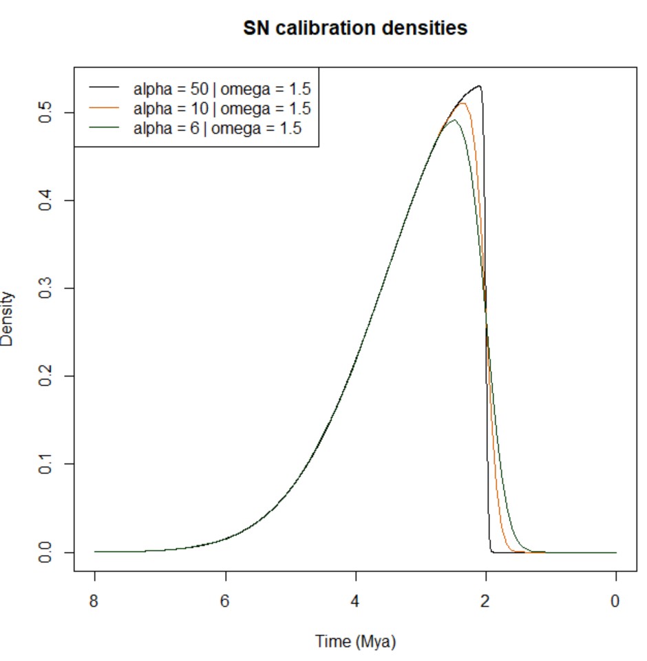
Skew-t distribution (ST($\xi, \omega, \alpha, \nu$); Azzalini and Genton 2008): the density of the skew-t distribution has an additional parameter to the SN distribution: the degree of freedom $\nu$. The density is the following:

$f_{ST}(x;\xi,\omega,\alpha,\nu)=\frac{2}{\omega}t(z;\nu)T(\alpha z\sqrt{(\nu+1)/(\nu+z^{2})};\nu+1)$

Eq. (9)

where $z=(x-\xi)/\omega$; $t$ and $T$ are the PDF and CDF of the standard t distribution, respectively, which are defined as follows:

$t(z;v)=\frac{\Gamma(\frac{1}{2}(\nu+1))}{\sqrt{\pi\nu}\Gamma(\frac{1}{2}\nu)}[1+\frac{z^{2}}{\nu}]^{-(\nu+1)/2}$
$$T(z;\nu)=\begin{cases} \frac{1}{2}I_{\nu/(\nu+z^{2})}(\frac{1}{2}\nu,\frac{1}{2}), & \textrm{if }z<0,\ 1-T(-z;\nu), & \textrm{if }z\geqslant0, \end{cases}$$

Eqs. (10 and 11)

NOTE: Eq. (11) does not seem to be displayed properly when written in that specific location (i.e., within a bullet point and following specific indentation). Please check the fully rendered Eq. (11) after the R code snippet below.

where $\Gamma()$ is the Gamma function and

$I_{p}(a,b)=\frac{1}{B(a,b)}\intop_{0}^{p}u^{a-1}(1-u)^{b-1}du$

Eq. (12)

is the incomplete Beta function ratio, or the CDF of the $Beta(a,b)$ distribution. However, the following

$B(a,b)=\intop_{0}^{1}u^{a-1}(1-u)^{b-1}du=\frac{\Gamma(a)\Gamma(b)}{\Gamma(a+b)}$

Eq. (13)

is the Beta function. Please note that you can also use the R package sn Azzalini 2023 to plot skew-t densities. As per the SN densities, it is harder to establish parameters $\omega$, $alpha$, and $\nu$ from scractch; it is easier to fit ST densities to a sample of time estimates (e.g., you may obtain them during MCMC). You may want to read Sandra Álvarez-Carretero's guidelines to fit SN/ST distributions -- you will find links to R scripts that you can adapt to analyse your own datasets.

Below, you can find an example of how to plot various ST densities with $\xi = 2$ and different values of $\nu$ (SN densities are overlapped for comparison):
```
par( mfrow = c( 1, 3 ) )
cols <- c( "#D55E00", "#023903" )
alpha  <- c( 50, 10, 6 )
nu     <- c( 1, 3, 2.2 )
for( i in seq(1, length(alpha) ) ){
    curve( sn::dsn( x, xi = 2, omega = 1.5, alpha = alpha[i] ),
          from = 0, to = 8, n = 1e4, xlim = rev( c( 0, 8 ) ),
          xlab = "Time (Mya)", ylab = "Density",
          main = "SN vs ST calibration densities",
          col = cols[1] )
    curve( sn::dst( x, xi = 2, omega = 1.5, alpha = alpha[i], nu = nu[i] ),
          col = cols[2], add = TRUE )
    legend( "topleft",  lty = 1, col = cols,
            legend = c( paste( "SN: alpha = ", alpha[i], " | omega = 1.5",
                              sep = "" ),
                        paste( "ST: alpha = ", alpha[i],
                              " | omega = 1.5 | nu = ",
                              nu[i], sep = "" ) ) )
}
```

Important

Eq. (11) properly rendered:

$$T(z;\nu)=\begin{cases} \frac{1}{2}I_{\nu/(\nu+z^{2})}(\frac{1}{2}\nu,\frac{1}{2}), & \textrm{if }z<0,\\\ 1-T(-z;\nu), & \textrm{if }z\geqslant0, \end{cases}$$

Note

Below, you can find some notes about ST and SN distributions:

When the shape parameter $\alpha = 0$, the distributions become the standard (symmetrical) normal and t distributions.
Changing $\alpha$ to $-\alpha$ flips the density at $x = \xi$ (the location parameter). Fossil calibrations should have long right tails, which means $\alpha > 0$. A larger $|(\alpha)|$ means more skewed distributions. When $|\alpha| = \infty$, the distribution is called folded normal or folded t distribution. In other words, the normal or t distribution truncated at $\xi$ from the left ($\alpha = \infty$) or from the right ($\alpha = -\infty$). When the degree of freedom $\nu = \infty$, the t or skew-t distribbution becomes the normal or skew normal distribution. The smaller $\nu$ is, the heavier the tails are. A small $\nu$ (e.g., values between 1 and 4) with a large shape parameter $\alpha$ in the skew-t distribution represents virtually hard minimum bound and very uncertain maximum bound. When $\nu = 1$, the t distribution is known as the Cauchy distribution, which does not have mean or variance. Both skew normal and skew-t distributions go from $-\infty$ to $\infty$. In MCMCtree, negative values are automatically truncated, so only the positive part is used. If feasible, please try to construct the distribution so that the probability for negative values is small (e.g., $<0.1%$). Please plots ST and SN densities using the template R code given above or Azzalini's website to check that the shape of your ST or SN distributions represent your knowledge of the fossil record and look sensible. In addition, if you are to fit ST or SN distributions to a sample of divergence times, you may want to read Sandra Álvarez-Carretero's guidelines to fit SN/ST distributions -- you will find links to R scripts that you can adapt to analyse your own datasets.

How to visualise your calibration densities?

Before timetree inference, you need to decide which distributions (and which shape!) may best represent your interpretation of the fossil record, which you shall use to constrain specific node ages on your fixed tree topology.

To easily visualise how your chosen calibration densities may look like, you can use the R package mcmc3r ([dos Reis et al. (2018)]). At the moment, you can use functions mcmc3r::dB, mcmc3r::dL, and mcmc3r::dU to plot soft-bound, low-bound, and upper-bound calibration densities, respectively. Below, you have a code snippet that you can use to plot some examples of such distributions:

# First, intsall the `devtools` and `mcmc3r`
# if you do not have them yet!
install.packages( "devtools" )
devtools::install_github( "dosreislab/mcmc3r" )

# Now, let's plot some examples!
# We will have a 3 rows and 2 columns to plot
# 2 examples for each type of calibration
# density you can plot with the `mcmc3r` 
# R package
# NOTE: The x axis will be reversed (i.e., from
# older to younger) so that it is
# easier to interpret the calibration densities
par( mfrow = c( 3, 2 ) )

# 1. Soft-bound calibration
#
# Example a)
#  - Minimum age is 6MY
#  - Maximum age is 8MY
#  - Both tail probabilities are soft (0.025)
#
# The code below plots the uniform distribution between
# 6MY and 8MY with soft bounds and two horizontal lines
# at 6MY and 8MY
curve( mcmc3r::dB( x, tL = 6, tU = 8, pL = 0.025, pU = 0.025 ),
       from = 4, to = 10, n = 1e4, xlim = rev( c( 4, 10 ) ),
       xlab = "Time (Mya)", ylab = "Density",
       main = "Soft minimum & maximum | 'B(6,8,0.025,0.025)'" )
abline( v = c( 6, 8 ), col = "#56B4E9" )

#
# Example b)
#  - Minimum age is 6MY
#  - Maximum age is 8MY
#  - Soft tail probability for the lower bound (pL = 0.025)
#    but hard upper bound (pU = 1e-300)
#
# The code below plots the uniform distribution between
# 6MY (hard minimum, pL = 1e-300) and 8MY (hard maximum,
# pU = 1e-300) as well as two horizontal lines
# at 6MY and 8MY
curve( mcmc3r::dB( x, tL = 6, tU = 8, pL = 1e-300, pU = 0.025 ),
       from = 4, to = 10, n = 1e4, xlim = rev( c( 4, 10 ) ),
       xlab = "Time (Mya)", ylab = "Density",
       main = "Hard minimum & soft maximum | 'B(6,8,1e-300,0.025)'" )
abline( v = c( 6, 8 ), col = "#56B4E9" )

# 2. Lower-bound calibration
#
# Example a)
#  - Minimum age is 1MY
#  - Offset p = 0.1
#  - Scale c = 0.2
#  - Soft lower bound pL = 0.025
#
# The code below plots a heavy-tailed density based
# on a truncated Cauchy distribution with a 
# soft minimum (pL = 0.025) at 1MY (parameter values
# set to p = 0.1 and c = 0.2); a horizontal line is also
# plotted at 1MY
curve( mcmc3r::dL( x, tL = 1, p = 0.1, c = 0.2, pL = 0.025 ),
       from = 0, to = 4, n = 1e4, xlim = rev( c( 0, 4 ) ),
       xlab = "Time (Mya)", ylab = "Density",
       main = "Soft minimum | 'L(1,0.1,0.2,0.025)'" )
abline( v = 1, col = "#56B4E9" )
#
# Example b)
#  - Minimum age is 1MY
#  - Offset p = 0.1
#  - Scale c = 0.2
#  - Hard lower bound pL = 1e-300
#
# The code below plots a heavy-tailed density based
# on a truncated Cauchy distribution with a 
# soft minimum (pL = 0.025) at 1MY (parameter values
# set to p = 0.1 and c = 0.2); a horizontal line is also
# plotted at 1MY
curve( mcmc3r::dL( x, tL = 1, p = 0.1, c = 0.2, pL = 1e-300 ),
       from = 0, to = 4, n = 1e4, xlim = rev( c( 0, 4 ) ),
       xlab = "Time (Mya)", ylab = "Density",
       main = "Hard minimum | 'L(1,0.1,0.2,1e-300)'" )
abline( v = 1, col = "#56B4E9" )

# 3. Upper-bound calibration
#
# Example a)
#  - Maximum age is 8MY
#  - Soft upper bound pU = 0.025
#
# The code below plots an upper-bound distribution
# with a soft maximum (pU = 0.025) at 8MY; a
# horizontal line is also plotted at 8MY
curve( mcmc3r::dU( x, tU = 8, pU = 0.025 ),
       from = 0, to = 9, n = 1e4, xlim = rev( c( 0, 9 ) ),
       xlab = "Time (Mya)", ylab = "Density",
       main = "Soft maximum | 'U(8,0.025)'" )
abline( v = 8, col = "#56B4E9" )
#
# Example b
#  - Maximum age is 8MY
#  - Hard upper bound pU = 1e-300
#
# The code below plots an upper-bound distribution
# with a hard maximum (pU = 1e-300) at 8MY; a
# horizontal line is also plotted at 8MY
curve( mcmc3r::dU( x, tU = 8, pU = 1e-300 ),
       from = 0, to = 9, n = 1e4, xlim = rev( c( 0, 9 ) ),
       xlab = "Time (Mya)", ylab = "Density",
       main = "Hard maximum | 'U(8,1e-300)'" )
abline( v = 8, col = "#56B4E9" )

If you run the code above, you should get the following plot:

You can use other in-built functions in R (or you can use your own scripts) to plot the densities when choosing Gamma, skew-t, or skew normal densities as shown in the section above.

Approximating the likelihood calculation

Thorne et al. (1998) suggested the use of the multivariate normal distribution of MLEs of branch lengths to approximate the likelihood function. To implement this approximation, one has to obtain the MLEs of the branch lengths and calculate their variance-covariance matrix or equivalently the matrix of second derivatives of the log likelihood with respect to the branch lengths (this matrix is also called the Hessian matrix). In Thorne’s multidivtime program, this is achieved using the program estbranches.

The approximation for the likelihood calculation implemented in MCMCtree (dos Reis and Yang 2011) has been found to be 1000x faster when compared to the exact likelihood calculation (Battistuzzi et al. 2011), and has been widely used in Bayesian node-dating analyses with phylogenomic data. For instance, it has been used in mammals (Meredith et al. 2011; dos Reis et al. 2012; Álvarez-Carretero et al. 2022), birds (Jarvis et al. 2014; Stiller et al. 2024), metazoans (dos Reis et al. 2015), and plants (Barba-Montoya et al. 2018; Morris et al. 2018); and also to study the origin of life on Earth (Betts et al. 2018; Moody et al. 2024).

How does this method work? Quick overview

The approximation to the likelihood calculation can be enabled by setting usedata = 3 in the control file. When using this option, MCMCtree will prepare three temporary files for each locus (i.e., control file tmp#.ctl, sequence alignment with site patterns tmp#.txt, and tree file tmp#.trees; where # corresponds to the number of each locus in the input sequence file); then invoke BASEML (if nucleotide data) or CODEML (if amino acid data) to calculate the MLEs of branch lengths and the Hessian matrix. E.g., if there was only one alignment block in the input sequence file, the three temporary files would be tmp0001.ctl, tmp0001.txt, and tmp0001.trees. Sometimes, some loci in the input sequence file (if more than one alignment block) may have missing taxa that are not present in the fixed tree topology given by the user in the input tree file. In such a case, the tree that will be written out for each locus in the corresponding output file tmp#.trees is generated by pruning the main tree (i.e., Newick tree in the input tree file) so that only those species present at the locus remain, and by unrooting the resulting tree.

Important

The tree saved in output file tmp#.trees should NOT be edited. Nevertheless, you may edit the relevant control file tmp#.ctl if you want to run another analysis by changing the substitution model under which BASEML (if nucleotide data) or CODEML (if amino acid) are to estimate the branch lengths, the gradient, and the Hessian. For instance, you may update variable method when working with large datasets and specify method = 1 to use a much more efficient algorithm (Yang 2000b). For more details on the iteration algorithms, please check the section below.

Note

If you open the tmp#.ctl, you will see that various options that you included in the main control file you wrote to run MCMCtree with usedata = 3 do not appear there: mcmcfile, clock, BDparas, rgene_gama, sigma2_gamma, print, burnin, sampfreq, nsample. The newly generated temporary control file will be used by CODEML (if amino acid data) or BASEML (if nucleotide data) to estimate the branch lengths, the gradient, and the Hessian; and so all variables concerning timetree inference are not listed as these programs do not use them. You will see that the only variables that are kept from the main control file you wrote are those that also work with CODEML and BASEML. E.g.: variables to specify the evolutionary model, the type of data used, and the paths to input files.

The output file out.BV from usedata = 3 should then be renamed to in.BV. This file has one block of results for each locus in the same order the alignment blocks are listed in the input sequence file (e.g., the first block of results would correspond to the first alignment block in the sequence file, and so on). If you manually edit the control file tmp#.ctl and then invoke BASEML or CODEML from the command line (for example, by typing codeml tmp0001.ctl), you will have to manually copy the content of rst1 into in.BV.

Important

If you are analysing large phylogenomic datasets and/or you have many alignment blocks in your input sequence file, using usedata = 3 as currently implemented may take a bit longer than you expect: CODEML (if amino acid data) or BASEML (if nucleotide data) will be called by MCMCtree to estimate the branch lengths, the gradient, and the Hessian for each locus (alignment block), one after the other. If you are using a HPC with wall time restrictions and you have many alignment blocks in your input sequence file, the jobs may get killed before all loci have been parsed! If that is your case, we suggest you follow the guidelines below, which show you how you can invoke BASEML or CODEML as aforementioned to speed the estimation of branch lengths, gradient, and Hessian for many loci:

a) Run MCMCtree with usedata = 3 until the three important temporary files are created (i.e., tmp#.ctl, tmp#.trees, and tmp#.txt), then stop the run by pressing ctrl+C in the terminal. You should press ctrl+C as soon as you see the following screen output:

*** Locus 1 ***
running codeml tmp0001.ctl

AAML in paml version 4.10.7, June 2023
ns = 7          ls = 469
Reading sequences, sequential format..
Reading seq # 7: gibbon
Sequences read..

469 site patterns read, 3331 sites
Counting frequencies..

   168 bytes for distance
 150080 bytes for conP
  18760 bytes for fhK
5000000 bytes for space

b) Once the temporary files are created (one per locus), variable method needs to be set to method = 1. The iteration algorithm enabled when selecting method = 1 is much more efficient with large datasets than the algorithm enabled when setting method = 0, and thus it is expected to finish quicker ([more details in the section below]).
c) Once the control files are edited, you can submit a job array to a HPC to simultaneously run CODEML (if amino acid data) or BASEML (if nucleotide data) for each loci so that the branch lengths, gradient, and Hessian are estimated simultaneously for each loci, thus saving much more time.
d) As aforementioned, you will then need to copy the content of each rst1 (one per locus) into a file called in.BV. Please make sure that you copy the results blocks in the same order as the alignment blocks appear in the input sequence file (i.e., the rst1 obtained when analysing the first locus should be the first results block in the in.BV, and so on).

[NOTE]: by also running CODEML or BASEML separately, you can modify the individual tmp#.ctl files so that different loci are analysed under different substitution models. The results block for each locus (alignment block) will have the branch lengths, gradient, and Hessian estimated under the corresponding substitution models, which will then be used in the next step by MCMCtree (i.e., usedata = 2 <path_to_inBV>) to approximate the likelihood calculation.

Once you have the in.BV file, you can then run MCMCtree again, now by changing variable usedata to usedata = 2 <path_to_inBV> in the main control file you first used. It is recommended you run timetree inference with MCMCtree in different folders from those you ran the steps described above; remember that output files are overwritten. You also need to run MCMCtree at least twice for each dataset so that you can check whether the chains have converged. When usedata = 3, MCMCtree reads the MLEs for the branch lengths, the gradient vector, and the Hessian matrix from the in.BV; then applies the approximate method for calculating the likelihood during the MCMC.

Note

You can have the in.BV file in the same folder as the control file or in a different location. If the latter, remember that you must specify the absolute or relative path to the in.BV in the control file as part of variable usedata; usedata = 2 <path_to_inBV>.

Note

In effect, option usedata = 3 in MCMCtree performs the function of estbranches from the multidivtime program. As aforementioned, you can always perform this step by running BASEML or CODEML externally once you obtain the three temporary files tmp#.ctl, tmp#.trees, and tmp#.txt. Similarly, option usedata = 2 approximates the likelihood calculation using the function of the multidivtime program.

Models of amino acid or codon substitution are NOT implemented in MCMCtree for the exact likelihood calculation, and so the only way to use those models is through the approximate method (usedata = 3 + usedata = 2 <path_to_inBV>). If is advisable that you edit the intermediate control file tmp#.ctl to choose the appropriate model of amino acid or codon substitution in the CODEML analysis, and then copy the results into the in.BV file as described in the section above.

Important

Please have a look at the estimated branch lengths in the tree when using this approach. If many of them are near 0, you should be concerned: you may have too little data or the tree is wrong for the locus.

Note

In this section, when referring to a "gene" or "locus" we refer to a "site partition" or "alignment block". For example, since the three codon positions typically have very different rates, different base compositions, etc., you may treat them as separate partitions and have different alignment blocks in your input sequence file.

The theory is described in detail in dos Reis and Yang 2011. The default transformation used to approximate the likelihood calculation in the program is the arcsin transformation. While not recommended, you can change the approximation by adding a third option to variable usedata: 1 for the square-root transformation, 2 for the logarithm transformation, and 3 for the arcsin transformation. E.g.: usedata = 2 <path_to_inBV> 3 uses the arcsin transformation (default).

How can you check that the approximation is reliable?

The iteration algorithm implemented in PAML uses the difference approximation to calculate derivatives, which is therefore used to calculate the Hessian matrix. The currently implemented method changes the variable ($x$) slightly in formula $df/dx = [f(x + e) - f(x)]/e$, say by a small number $e$, to see how the function value changes. Number $e$ should be small to allow accurate approximation, BUT not too small to avoid rounding errors. You can check whether the results are stable when running CODEML (if amino acid data) or BASEML (if nucleotide data) by changing the value of number $e$ by updating variable Small_Diff in the relevant control file tmp#.ctl generated by MCMCtree when setting usedata = 3, e.g., you may use Small_Diff = 1e-6. Please note that the iteration algorithm is rather sensitive to the value of number $e$. This chosen value also affects the calculation of the S.E.s for model parameters (only printed if specified in the control file with variable getSE; not needed for this type of approximation), which are much more difficult to approximate than the first derivatives. If the calculated S.E.s are sensitive to slight change in this variable, they are not reliable.

Note

If you compile the source code, you can also change the lower and upper bounds for model parameters as you cannot change them via the control file.

At the time of writing, there are two iteration algorithms implemented in PAML:

Option method = 0: the first algorithm, which can be enabled by setting method = 0 in the control file, is a general-purpose minimization algorithm that deals with upper and lower bounds for parameters but not general equality or inequality constraints. The algorithm requires first derivatives, which are calculated using the difference approximation, and accumulates information about the curvature (second derivatives) during the iteration using the BFGS updating scheme. At each iteration step, it calculates a search direction, and does a one-dimensional search along that direction to determine how far to go. At the new point, the process is repeated, until there is no improvement in the log-likelihood value, and changes to the parameters are very small. The algorithm updates all parameters, including branch lengths, simultaneously.
Option method = 1: the second algorithm, which can be enabled by setting method = 1 in the control file, works if an independent rate is assumed for each branch (i.e., use clock = 0 in CODEML [amino acid data] or BASEML [nucleotide data]) (see Yang 2000b for details). This algorithm cycles through two phases. During phase I, this method estimates branch lengths with substitution parameters fixed (e.g., parameters such as the transition/transversion rate ratio $\kappa$ or the gamma shape parameter $\alpha$). During phase II, the algorithm estimates substitution parameters using the BFGS algorithm mentioned above with branch lengths fixed. The procedure is repeated until the algorithm converges. In phase I of the algorithm, branch lengths are optimised one at a time. The advantage of the algorithm is that, when the likelihood is calculated for different values of one single branch length, as required when that branch length only is optimised, much of the likelihood calculations on the phylogeny is the same and can be avoided by storing intermediate results in the computer memory. A cycle is completed after all branch lengths are optimised. As estimates of branch lengths are correlated, several cycles are needed to achieve convergence of all branch lengths in the tree, that is, to complete phase I of the algorithm.

Important

If branch lengths are the only parameters to be estimated, that is, if substitution parameters are fixed, the second algorithm (method = 1) is much more efficient. The second algorithm is also more efficient if the data contain many sequences so that the tree has many branch lengths, which is why such an option should be enabled when using large phylogenomic datasets.

Main resources and citations

Approximate likelihood calculation for Bayesian estimation of divergence times
dos Reis M and Yang Z (2011). Approximate likelihood calculation for Bayesian estimation of divergence times. Mol. Biol. Evol. 28, 2161-2172.

This is the paper you need to cite if you are enabling the approximate likelihood calculation when using MCMCtree. All the theoretical and technical background required to understand the validation and implementation of such an approach are explained in this paper.
Bayesian Molecular Clock Dating Using Genome-Scale Datasets
dos Reis M and Yang, Z (2019). Bayesian Molecular Clock Dating Using Genome-Scale Datasets. In: Anisimova, M. (eds) Evolutionary Genomics. Methods in Molecular Biology, vol 1910. Humana, New York, NY.

If you want to learn how to analyse phylogenomic datasets with MCMCtree, this is the protocol paper you have been looking for! By following the step-by-step guidelines detailed in this protocol, you will learn how to make the most of the approximate likelihood calculation implemented in MCMCtree to analyse your large datasets. All input and control files required to follow the examples given in the protocol paper can be accessed via the divtime GitHub repository.

Important

Remember to not only go through the protocol paper, but also clone the divtime GitHub repository maintained by Mario dos Reis to access all input and control files that are used for the examples given in the protocol paper.

Dating Microbial Evolution with MCMCtree
dos Reis M (2022) Dating Microbial Evolution with MCMCtree. In: Haiwei Luo (ed.) Environmental Microbial Evolution: Methods and Protocols. Methods in Molecular Biology, vol 2569. Humana, New York, NY.

If you are planning on inferring microbial evolutionary timelines with MCMCtree while enabling the approximate likelihood calculation with amino acid data, you may want to take a look at this protocol! Example datasets and control files are described in detail and also made available on the microdiv GitHub repository.

Important

Remember to not only go through the protocol paper, but also clone the microdiv GitHub repository maintained by Mario dos Reis to access all input and control files that are used for the examples given in the protocol paper.

Enabling tip-dating analyses with `MCMCtree`

This option is specified by the following line in the control file:

TipDate = 1 100 * TipDate (1) & time unit

The example data file is in the examples/TipDate.HIV2/. When you run the default analysis, you will see the following printout on the monitor:

TipDate model
Date range: (1995.00, 1982.00) => (0, 0.13). TimeUnit = 100.00.

The end of each sequence name (see input file HIV2ge.txt) has the sampling year, which goes from 1994 to 1956.

Note

For instance, the first sequence identifier (e.g., sequence name) in the example sequence file is P03h and the year of sampling is 1995. Therefore, the first tag identifier is P03h1995.

According to the example data, the most recent sequence date is 1994 and the oldest is 1982. Given that time goes backwards in evolutionary timelines (from the most recent time to the oldest), we can set 1994 (earliest sampling time) to 0. The difference between the earliest and the oldest sampling times is 13, and thus the oldest sequence will have age 0.13 given that 1982 is 13 years earlier than 1994 and one time unit is specified to be 100 years.

Important

Remember that time unit can be controlled using variable TipDate as shown above.

The rest of the variables in the control file to run MCMCtree work in the same way as in the case of dating species divergence using fossil calibrations as node age constraints.

The root age prior is believed to be important, so please use the sample dates and time unit to specify the bounds on the rate age. Ideally, you should use whatever biological information available to specify the priors. For the example dataset mentioned above, a soft uniform density for the root age in the interval (1914, 1874) with tail probability $10^–10$ on both the left and right tails could be specified as B(0.8, 1.2, 1e-10, 1e-10); which would result in a uniform density yet quite sharp on the bounds. Please note that the root age constraint should be included in the input tree file.

Similarly, the prior on the mutation rate (i.e., prior specified using variable rgene_gamma in the control file) is also important. Remember that relaxed-lock models cane be specified setting variable clock to clock = 2 (independent-rates log-normal relaxed-clock model) or clock = 3 (autocorrelated-rates relaxed-clock model); while clock = 1 enables the strict clock model.

The newly implemented prior of times for tip-dating analyses is based on Tanja Stadler’s birth-death-sequential-sampling (BDSS) model, and the implementation in MCMCtree is described in Stadler and Yang 2013.

Important

Please note that, when the prior of times is used to date the divergences of viral sequences with sample dates, as shown in the example above and by Stadler and Yang 2013, you should use $\rho=0$ and $\psi > 0$ (i.e., third and fourth options in variable BDparas, respectively). When the BDSS prior is used to date species divergences, suc as to analyse fossil occurrence data to derive calibration densities (Wilkinson et al. 2011), one should have $\rho > 0$ and $\psi > 0$.

Please note that you should explore the densities that are derived when changing parameters lambda, mu, rho, and psi for the BDSS model to assess the impact that your specified prior may have on posterior mean time estimates:

BDparas = 2 1 0 0.8 * lambda, mu, rho, psi for the BDSS prior

Additional resources and `MCMCtree` applications

Bayesian model selection analyses

Bayesian model selection with MCMCtree and the R package mcmc3r was first described by dos Reis et al. (2018). Both the thermodynamic integration (e.g., Gelman and Meng 1998; Lartillot and Philippe 2006; Lepage et al. 2007) and the stepping-stone approach (Xie et al. 2011) have been implemented in the mcmc3r R package to prepare the input files that MCMCtree will require to sample from the relevant power posteriors.
A very detailed tutorial explaining how to use the functions in the mcmc3r R package to generate the file structure and input files required by MCMCtree to sample from the power posteriors has been written by Mario dos Reis. The mcmc3r R package and MCMCtree have been used in various types of Bayesian model selection analyses, such as those aiming to find the best-fitting relaxed-clock model (e.g., dos Reis et al. 2018; Álvarez-Carretero et al. 2019; McGowen et al. 2020) or the best-fitting tree topology (Perri et al., 2021).

RESOURCES AND CITATIONS

Using phylogenomic data to explore the effects of relaxed clocks and calibration strategies on divergence time estimation: Primates as a test case
dos Reis M, et al. (2018). Using phylogenomic data to explore the effects of relaxed clocks and calibration strategies on divergence time estimation: Primates as a test case. Syst. Biol. 67, 594–615.

Important

Remember to cite the mcmc3r R package if you use it (see tutorial via this link).

Bayesian timetree inference with continuous morphological data

The dating program MCMCtree can also be used to infer species divergence times using morphological quantitative data such as geometric morphometrics (GMM) data. Sandra Álvarez-Carretero and Mario dos Reis wrote a very detailed tutorial explaining how to parse the data in R, how to generate the morphological alignment and format it for MCMCtree, and how to enable the analysis of GMM data in MCMCtree.

RESOURCES AND CITATIONS

Bayesian estimation of species divergence times using correlated quantitative characters
Álvarez-Carretero S, et al. (2019). Bayesian estimation of species divergence times using correlated quantitative characters. Syst. Biol. 68, 967–986.

Important

Remember to cite the mcmc3r R package if you use it alongside MCMCtree to analyse morphological quantitative data. An example of how to obtain the morphological alignment ready to be used by MCMCtree is given in this R markdown tutorial.

Bayesian sequential subtree (BSS) approach

Sometimes, approximating the likelihood calculation (dos Reis and Yang 2011) may not be enough to infer evolutionary timelines within a reasonable amount of time when using very large genomic datasets. In such instances, the BSS approach can be of help!

A Bayesian sequential approach to tackle this issue was first used by Álvarez-Carretero et al. (2022), who validated and applied this method to infer a species-level timeline of mammal evolution with a phylogenomic dataset consisting of 4,705 mammal species. Sandra Álvarez-Carretero wrote a step-by-step tutorial that guides users through all the steps that were followed from data filtering to timetree inference with the aim to allow for reproducibility. Such a tutorial is available in the mammals_dating GitHub repository that Sandra created and maintains, where you shall find in-house scripts, input/intermediate/output files, control files, plots, links to download files too large to store on GitHub... Everything you may need to reproduce the results reported in the study!

RESOURCES AND CITATIONS

A species-level timeline of mammal evolution integrating phylogenomic data
Álvarez-Carretero S, et al. (2022) A species-level timeline of mammal evolution integrating phylogenomic data. Nature 602, 263–267.

Important

Remember to follow the guidelines in the step-by-step tutorial in the mammals_dating GitHub repository maintained by Sandra Álvarez-Carretero to reproduce the analyses detailed in the paper.

Cross-bracing (or equality constraints)

If you are working with deep phylogenies, you may have found yourself struggling to find fossil evidence to constrain the node age constraints of your tree topology. Such a scenario can lead to unbalanced calibrated tree topologies, which tend to cause problems during Bayesian timetree inference. If you have the chance to obtain paralogous sequences, however, you may have the chance to increase the number of nodes which age you constrain by using equality constraints, also known as cross-bracing.
Equality constraints have now been implemented, tested, and validated in MCMCtree (Moody et al. 2024), which can be helpful when the scarcity of the fossil for the taxa of interest leads to unbalanced calibrated tree topologies. By using paralogous genes, one can take advantage of duplication events, and thus find nodes in each duplicated node that correspond to the same speciation event. If such nodes are found, one can "flag" them to enforce equality constraints: during MCMC, sampling will not be independent; the same posterior time densities will be inferred for those nodes identified with the same flag. The documentation above includes all the details required to enable this type of node age constraints by including variable duplication in the control file and using a specific notation to identify relevant nodes in the input tree file.

For an example of how to use equality constraints in deep phylogenies, one can go through LUCA-divtimes GitHub repository to check the various timetree inference analyses Sandra Álvarez-Carretero carried out when inferring the age of LUCA as part of (Moody et al. 2024). Users can clone this repository to navigate the file structure and check all the README files, where extensive documentation and justifications for each analyses have been given. Users can also find in-house scripts to run PAML programs in a HPC (some settings may need to be adapted depending on the scheduler used) and carry out MCMC diagnostics in R. Explanations to enable equality constraints in MCMCtree, as well as in-house scripts to calibrate the tree topology in MCMCtree format, are also provided in the repository.

RESOURCES AND CITATIONS

The nature of the Last Universal Common Ancestor and its impact on the early Earth system
Moody et al. (2024) The nature of the last universal common ancestor and its impact on the early Earth system. Nat Ecol Evol 8, 1654-1666.

Important

Remember to follow the step-by-step tutorial available in the LUCA-divtimes GitHub repository maintained by Sandra Álvarez-Carretero to reproduce the analyses detailed in the paper.

If you use or adapt the LUCA-divtimes protocol (including the in-house scripts) for your analyses, please also cite the following:

Sandra Álvarez-Carretero. (2024). sabifo4/LUCA-divtimes: v1.0.1 (LUCAdivtimes-v1.0.1). Zenodo. https://doi.org/10.5281/zenodo.12731583

The software package is provided "as is" without warranty of any kind. In no event shall the author or their employer be held responsible for any damage resulting from the use of this software, including but not limited to the frustration that you may experience in using the package. The program package, including source codes, example data sets, executables, and this documentation is maintained by Ziheng Yang and distributed under the GNU GPL v3.

Ziheng Yang
Department of Genetics, Evolution, and Environment
University College London
Gower Street
WC1E 6BT, London, United Kingdom

Provide feedback

Saved searches

Use saved searches to filter your results more quickly

MCMCtree

MCMCtree

Overview

Control file

Older variables

Calibrations: how to set up node age constraints?

How to visualise your calibration densities?

Approximating the likelihood calculation

How does this method work? Quick overview

How can you check that the approximation is reliable?

Main resources and citations

Enabling tip-dating analyses with `MCMCtree`

Additional resources and `MCMCtree` applications

Bayesian model selection analyses

Bayesian timetree inference with continuous morphological data

Bayesian sequential subtree (BSS) approach

Cross-bracing (or equality constraints)

Uh oh!

Uh oh!

Uh oh!

Uh oh!

Uh oh!

Uh oh!

Uh oh!

Uh oh!

Uh oh!

Uh oh!

Uh oh!

Clone this wiki locally

MCMCtree

MCMCtree

Overview

Control file

Older variables

Calibrations: how to set up node age constraints?

How to visualise your calibration densities?

Approximating the likelihood calculation

How does this method work? Quick overview

How can you check that the approximation is reliable?

Main resources and citations

Enabling tip-dating analyses with MCMCtree

Additional resources and MCMCtree applications

Bayesian model selection analyses

Bayesian timetree inference with continuous morphological data

Bayesian sequential subtree (BSS) approach

Cross-bracing (or equality constraints)

Uh oh!

Uh oh!

Uh oh!

Uh oh!

Uh oh!

Uh oh!

Uh oh!

Uh oh!

Uh oh!

Uh oh!

Uh oh!

Clone this wiki locally

Enabling tip-dating analyses with `MCMCtree`

Additional resources and `MCMCtree` applications