Ploting POINT sf with geom_sf() is slow #2718
Comments
|
Could you check whether there is any relation to issue #2655? |
|
Thanks, I roughly think this is a different issue because I'm using Windows (sorry I forgot to write this). But, I will check further. |
|
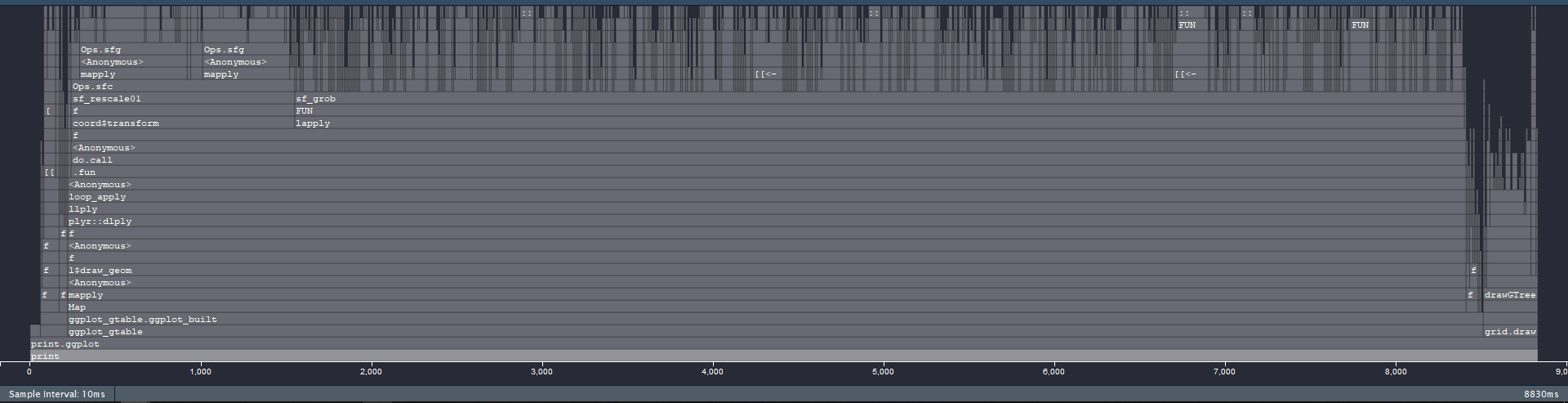
Here's the result of profvis of the code that plots 1000
|
|
Here's a reprex. This shows library(ggplot2)
library(sf)
#> Linking to GEOS 3.6.1, GDAL 2.2.3, proj.4 4.9.3
set.seed(1)
n <- 1000
d <- data.frame(
x = runif(n) * 360,
y = runif(n) * 180
)
d_sf <- st_multipoint(as.matrix(d)) %>%
st_sfc() %>%
st_cast("POINT")
system.time({
p <- ggplot(d_sf) +
geom_sf()
print(p)
})Created on 2018-06-28 by the reprex package (v0.2.0). Session infodevtools::session_info()
#> ─ Session info ──────────────────────────────────────────────────────────
#> setting value
#> version R version 3.5.0 (2018-04-23)
#> os Windows 10 x64
#> system x86_64, mingw32
#> ui RTerm
#> language (EN)
#> collate Japanese_Japan.932
#> tz Asia/Tokyo
#> date 2018-06-28
#>
#> ─ Packages ──────────────────────────────────────────────────────────────
#> package * version date source
#> assertthat 0.2.0 2017-04-11 CRAN (R 3.5.0)
#> backports 1.1.2 2017-12-13 CRAN (R 3.5.0)
#> bindr 0.1.1 2018-03-13 CRAN (R 3.5.0)
#> bindrcpp 0.2.2 2018-03-29 CRAN (R 3.5.0)
#> callr 2.0.4 2018-05-15 CRAN (R 3.5.0)
#> class 7.3-14 2015-08-30 CRAN (R 3.5.0)
#> classInt 0.2-3 2018-04-16 CRAN (R 3.5.0)
#> cli 1.0.0 2017-11-05 CRAN (R 3.5.0)
#> clisymbols 1.2.0 2017-05-21 CRAN (R 3.5.0)
#> colorspace 1.3-2 2016-12-14 CRAN (R 3.5.0)
#> crayon 1.3.4 2017-09-16 CRAN (R 3.5.0)
#> curl 3.2 2018-03-28 CRAN (R 3.5.0)
#> DBI 1.0.0 2018-05-02 CRAN (R 3.5.0)
#> debugme 1.1.0 2017-10-22 CRAN (R 3.5.0)
#> desc 1.2.0 2018-05-01 CRAN (R 3.5.0)
#> devtools 1.13.5.9000 2018-05-17 Github (r-lib/devtools@13ee56b)
#> digest 0.6.15 2018-01-28 CRAN (R 3.5.0)
#> dplyr 0.7.5 2018-05-19 CRAN (R 3.5.0)
#> e1071 1.6-8 2017-02-02 CRAN (R 3.5.0)
#> evaluate 0.10.1 2017-06-24 CRAN (R 3.5.0)
#> ggplot2 * 2.2.1.9000 2018-06-26 Github (tidyverse/ggplot2@348b26f)
#> glue 1.2.0 2017-10-29 CRAN (R 3.5.0)
#> gtable 0.2.0 2016-02-26 CRAN (R 3.5.0)
#> htmltools 0.3.6 2017-04-28 CRAN (R 3.5.0)
#> httr 1.3.1 2017-08-20 CRAN (R 3.5.0)
#> knitr 1.20.2 2018-05-10 local
#> lazyeval 0.2.1 2017-10-29 CRAN (R 3.5.0)
#> magrittr 1.5 2014-11-22 CRAN (R 3.5.0)
#> memoise 1.1.0 2018-06-13 Github (hadley/memoise@06d16ec)
#> mime 0.5 2016-07-07 CRAN (R 3.5.0)
#> munsell 0.5.0 2018-06-12 CRAN (R 3.5.0)
#> pillar 1.2.3 2018-05-25 CRAN (R 3.5.0)
#> pkgbuild 1.0.0 2018-05-17 Github (r-lib/pkgbuild@0457039)
#> pkgconfig 2.0.1 2017-03-21 CRAN (R 3.5.0)
#> pkgload 1.0.0 2018-05-17 Github (r-lib/pkgload@35efedd)
#> plyr 1.8.4 2016-06-08 CRAN (R 3.5.0)
#> processx 3.1.0 2018-05-15 CRAN (R 3.5.0)
#> purrr 0.2.5 2018-05-29 CRAN (R 3.5.0)
#> R6 2.2.2 2017-06-17 CRAN (R 3.5.0)
#> Rcpp 0.12.17 2018-05-18 CRAN (R 3.5.0)
#> rlang 0.2.1 2018-05-30 CRAN (R 3.5.0)
#> rmarkdown 1.10 2018-06-11 CRAN (R 3.5.0)
#> rprojroot 1.3-2 2018-01-03 CRAN (R 3.5.0)
#> scales 0.5.0.9000 2018-06-26 Github (hadley/scales@9e5e4d4)
#> sessioninfo 1.0.0 2017-06-21 CRAN (R 3.5.0)
#> sf * 0.6-3 2018-05-17 CRAN (R 3.5.0)
#> spData 0.2.9.0 2018-06-17 CRAN (R 3.5.0)
#> stringi 1.2.3 2018-06-12 CRAN (R 3.5.0)
#> stringr 1.3.1 2018-05-10 CRAN (R 3.5.0)
#> testthat 2.0.0 2017-12-13 CRAN (R 3.5.0)
#> tibble 1.4.2 2018-01-22 CRAN (R 3.5.0)
#> tidyselect 0.2.4 2018-02-26 CRAN (R 3.5.0)
#> units 0.6-0 2018-06-09 CRAN (R 3.5.0)
#> usethis 1.3.0 2018-02-24 CRAN (R 3.5.0)
#> withr 2.1.2 2018-06-26 Github (jimhester/withr@fe56f20)
#> xml2 1.2.0 2018-01-24 CRAN (R 3.5.0)
#> yaml 2.1.19 2018-05-01 CRAN (R 3.5.0) |


|
Here's a rough implementation for this. Does this make sense? If so, I will try to make the code ready to merge. (Sorry, I just wanted to make a PR on my repo to show codes, but I mistakenly created here... 🙄 ) https://github.com/tidyverse/ggplot2/pull/2722/files |
|
Furthermore |
|
Personally I’m not sure if it is the goal of ggplot2 to optimise the input data. It might lead to unexpected results, e.g. in the stacking order of the different features... If a fail-safe approach could be found it might be worth it but otherwise just documenting that multiple POINT will render slowly... There’s no problem combining geom_sf and geom_point btw |
|
Basically I agree with @thomasp85, but I feel this is unacceptably slow and should be fixed. In the case of #2655, it was not the ggplot2's fault and it seems there's nothing we can do. But, in this case, considering That said, I don't think my PR is a good way to fix this. Maybe is it better to implement |
|
At some point, we may have to bite the bullet and see if we can speed up grid. It seems absurd that we cannot draw thousands of points as individual grobs without experiencing extreme speed penalties. The same applies to drawing many individual text labels. Otherwise we will have to keep making design choices in ggplot2 that are driven by limitations of grid rather than by what would be a clean design. E.g., I find this comment on |
|
I agree - as I’ve stated before I really hope to get some time to review the whole stack with performance in mind My problem in combining POINT to multipoint is that it will result in all points being the same colour - also if a line or polygon were mixed in with the points, it would loose its ordering in the drawing stack |
|
Hmm, thanks. I didn't notice the point that we can speed up grid. It's reasonable to wait for it and avoid adding complex tweaks. OK, please close this issue anytime. One thing, this is NOT true, if you are talking about combining POINTs in ggplot2:
If this is about combining them outside ggplot2, you are right. That's why I felt this should happen inside |
|
Sorry, may I confirm one more thing? I wonder if this is really true.
As I showed above (#2718 (comment)), most of the time is spent for |
|
I‘ve experienced the performance hit in the drawing, not the building stage. |
|
I think many things are slow. If I look at the code for Considering that ultimately all microbenchmark::microbenchmark(
grid::gpar(color = "blue"), list(color = "blue")
)
#> Unit: nanoseconds
#> expr min lq mean median uq max
#> grid::gpar(color = "blue") 18715 19526 220562.0 20031.0 21431.5 19759145
#> list(color = "blue") 143 161 308.2 185.5 217.0 8740
#> neval
#> 100
#> 100Created on 2018-06-28 by the reprex package (v0.2.0). |
|
Another example. I realize that my code reorders the list, but that may or may not matter. For aesthetics or other graphical parameters that are always named it doesn't matter. And I bet by implementing the entire function in C++ we could have similar or better speed without the reordering problem. (Not sure why the maximum is so high though for update_list <- function(old, new) {
names_new <- names(new)
names_old <- names(old)
old[intersect(names_old, names_new)] <- NULL
c(old, new)
}
l1 <- list(a = 1, b = 2, c = 3)
l2 <- list(a = 5, c = 3, d = 4)
update_list(l1, l2)
#> $b
#> [1] 2
#>
#> $a
#> [1] 5
#>
#> $c
#> [1] 3
#>
#> $d
#> [1] 4
utils::modifyList(l1, l2)
#> $a
#> [1] 5
#>
#> $b
#> [1] 2
#>
#> $c
#> [1] 3
#>
#> $d
#> [1] 4
microbenchmark::microbenchmark(
update_list(l1, l2),
utils::modifyList(l1, l2)
)
#> Unit: microseconds
#> expr min lq mean median uq
#> update_list(l1, l2) 7.202 8.393 215.79596 9.3245 10.4400
#> utils::modifyList(l1, l2) 33.227 35.609 38.01464 37.4455 38.8585
#> max neval
#> 20604.255 100
#> 77.789 100Created on 2018-06-28 by the reprex package (v0.2.0). |
|
I just wanted to loop @tmastny in here. We're both interested in improving performance and have been recently profiling ggplot2 and grid code. Helpfully Tim has more background in compiled code than I do. Likely this thread is not the place to organize them but Tim and I would be happy to talk more about known slowpoints or a wishlist of things to investigate. |
|
One more example. Just by circumventing grid error checking and creating grobs directly we can get a ~3 fold speed increase for points. library(grid)
library(purrr)
library(dplyr)
# fast version of gpar
gpar_fast <- function(...) {
structure(
list(...),
class = "gpar"
)
}
# fast version of pointsGrob()
pointsGrob_fast <- function(xu = unit(0.5, "native"), yu = unit(0.5, "native"),
pch = 1, size = unit(1, "char"),
name = "none", gp = gpar_fast(), vp = NULL) {
structure(
list(
x = xu,
y = yu,
pch = as.integer(pch),
size = size,
name = name,
gp = gp,
vp = vp
),
class = c("points", "grob", "gDesc")
)
}
# fast and slow grobs are identical
identical(
pointsGrob_fast(unit(0.5, "npc"), unit(0.5, "npc"), name = "none"),
pointsGrob(unit(0.5, "npc"), unit(0.5, "npc"), name = "none")
)
#> [1] TRUE
n <- 50
df <- tibble(
x = runif(n),
y = runif(n),
color = sample(c("red", "green", "blue"), n, replace = TRUE)
) %>% mutate(
xu = map(x, ~unit(.x, "native")),
yu = map(y, ~unit(.x, "native")),
)
# standard grid
f1 <- function() {
pmap(
df,
function(x, y, color, ...) {
gp <- gpar(col = color)
pointsGrob(x, y, gp = gp)
}
)
}
# fast points, slow gpar
f2 <- function() {
pmap(
df,
function(xu, yu, color, ...) {
gp <- gpar(col = color)
pointsGrob_fast(xu, yu, gp = gp)
}
)
}
# fast points, fast gpar
f3 <- function() {
pmap(
df,
function(xu, yu, color, ...) {
gp <- gpar_fast(col = color)
pointsGrob_fast(xu, yu, gp = gp)
}
)
}
# plot output is the same
grid.newpage()
pushViewport(viewport())
grid.draw(do.call(gList, f1()))grid.newpage()
pushViewport(viewport())
grid.draw(do.call(gList, f3()))microbenchmark::microbenchmark(
f1(),
f2(),
f3(),
times = 50
)
#> Unit: milliseconds
#> expr min lq mean median uq max neval
#> f1() 6.785814 6.999505 8.152342 7.623538 9.108686 12.428292 50
#> f2() 2.305470 2.485765 3.349848 2.674786 3.282183 11.510736 50
#> f3() 1.866726 1.994537 2.521616 2.113111 2.633927 6.555309 50Created on 2018-06-28 by the reprex package (v0.2.0). |


|
Thanks so much for the nice codes and explanations!
I didn't notice that, but you are right. In fact, my profvis shows
But, for
I'm not sure if this is the typical performance issue of ggplot2, but I'm happy to keep this issue open for that kind of discussion. 👍 |

|
I understand less about ggplot2 internals than the other members of this thread, but just in case this says anything useful about implementation / communication with graphics devices, I ran a recent performance benchmark comparing ggplot2 rendering to tmap -- Plotting the same plot using the same spatial point data & graphics device (RStudioGD macOS / Quartz), rendering the tmap plot was 80x faster but also used an 80x larger object. |
|
I believe this is closed by #3164 👍 |
|
This old issue has been automatically locked. If you believe you have found a related problem, please file a new issue (with reprex) and link to this issue. https://reprex.tidyverse.org/ |
Uh oh!
There was an error while loading. Please reload this page.
In my environment, it takes 10 seconds for plotting 1000
POINTs bygeom_sf().I feel this is a bit too long for exploring the data.
https://gist.github.com/yutannihilation/479cb5f254826915a7a3d36ff84b4b43
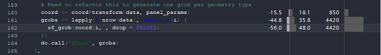
I suspect this is because
draw_panel()appliessf_as_grob()on every row. Is it possible to do this more efficiently, e.g.st_combine()pergroupso that it plots oneMULTIPOINTthat contains 1000 points?The text was updated successfully, but these errors were encountered: